21.1 Reinstein: What is the goal of statistical analysis?
Modern econometrics mainly focuses on the (causal) identification and estimation of a single parameter or ‘treatment effect’.1 Economists often make choices to make the identification of this parameter more robust (e.g., identified under weaker assumptions) or more efficient — even if this tends to make the overall model worse at predicting the outcomes. E.g., they may leave out a possibly variable that is possibly ‘endogenous’ in a way that could bias the estimate of the parameter of interest, even if it is clear that in increases the predictive power of the model.
Econometrics also focuses a lot on the unbiasedness of parameter estimates.2 One justification for focusing on unbiasedness might be in the context of a judge in an adversarial proceeding; even if it may be a bad predictor, we know this estimate does not understate or overstate an effect on average; thus it favors neither side of the debate.
Perhaps for these reasons (focus on a single parameter, concern for unbiasedness), econometricians seem reluctant t use random effects/mixed models and ‘regularization’. Where they use these, I think it is often only for ‘incidental parameters’, not for the parameters of interest. I recall that the classic ‘Stein shrinkage estimator’ is a better predictor (in terms of mean squared error) but it is not unbiased. Similarly, if we ‘regularize’ an estimate of a ‘necessary control’3 the estimated parameter on our regressor of interest may be biased.
My potential concern: I’m not sure McElreath is always clear on how he sees as the goal of statistical analysis, and how it informs scientific knowledge. (Of course, at RP we have practical goals, not just the expansion of knowledge for its own sake.) When a model ‘fits the outside data better’ i.e., it ‘predicts better’, does it necessarily ‘represent the truth about the question of interest better’? Perhaps it is focusing too little on the relationship of greatest interest, in favor of finding a model that fits better overall.
Relatedly, he seems to be somewhat interested in ‘falsification done right’. But it’s not clear to me how his take on a Bayesian framework does this. In particular, in some of the causal chapters, it seems like he is suggesting a DAG can be falsified by something that seems to me like an ‘absence of evidence of a relationship’, rather than, e.g., an equivalence test or a posterior tightly bounded around 0.
21.2 Statistical golems
” Scientists also make golems… scientific models.”
But these golems have real effects on the world, through the predictions they make and the intuitions they challenge or inspire. A concern with truth enlivens these models, but just like a golem or a modern robot, scientific models are neither true nor false, neither prophets nor charlatans. Rather they are constructs engineered for some purpose. These constructs are incredibly powerful, dutifully conducting their programmed calculations.
Kurz: one of the most powerful themes interlaced throughout the pages is how we should be skeptical of our models. McElreath presentation?
21.3 Hostility to cookbooks and flowcharts
Advanced courses in statistics do emphasize engineering principles, but most scientists never get that far. Teaching statistics this way is somewhat like teaching engineering backwards, starting with bridge building and ending with basic physics
Why aren’t the tests enough for research? The classical procedures of introductory statistics tend to be inflexible and fragile. By inflexible, I mean that they have very limited ways to adapt to unique research contexts. By fragile, I mean that they fail in unpredictable ways when applied to new contexts
Fisher’s exact test, which applies (exactly) to an extremely narrow empirical context, but is regularly used whenever cell counts are small
… ethinking statistical inference as a set of strategies, instead of a set of pre-made tools.
21.4 Null hypothesis significance testing and falsification
Paraphrasing from McElreath’s lecture video:
Scientists have turned things upside down; originally the idea was that you had substantive of hypotheses that you would want to falsify and now we try to falsify silly null hypotheses that “nothing is going on”. You should try to really build a hypothesis and test it not just reject that nothing is going on.
greatest obstacle that I encounter among students and colleagues is the tacit belief that the proper objective of statistical inference is to test null hypotheses
deductive falsification is impossible in nearly every scientific context
Intricate argument for this, non-unique predictions of models
Many models correspond to the same hypothesis, and many hypotheses correspond to a single model. This makes strict falsification impossible. (2) Measurement matters. Even when we think the data falsify a model, another observer will debate our methods and measures. They don-t trust the data. Sometimes they are right.
All models are false, so what does it mean to falsify a model? One consequence of the requirement to work with models is that it’s no longer possible to deduce that a hypothesis is false, just because we reject a model derived from it.
And so this fact yields a statistical model, MII, that predicts a power law in the data. In contrast the constant selection process model P1A predicts something quite different, MIII. Unfortunately, other selection models (P1B) imply the same statistical model, MII, as the neutral model. They also produce power laws
If we reject the null, we can’t really conclude that selection matters, because there are other neutral models that predict different distributions of alleles. And if we fail to reject the null, we can’t really conclude that evolution is neutral, because some selection models expect the same frequency distribution
What about ‘black swan’ falsification?:
we most often face two simultaneous problems that make the swan fable misrepresentative. First, observations are prone to error, especially at the boundaries of scientific knowledge. Second, most hypotheses are quantitative, concerning degrees of existence, rather than discrete, concerning total presence or absence
H0 “Black swans are rare”
Neutrinos case:
the “measurement” in this case is really an estimate from a statistical model, all false and true positives are possible..? usually measurement error is an issue. so black swan falsification is not so simple
Rethinking: Is NHST falsificationist?
Null hypothesis significance testing, NHST, is often identified with the falsificationist, or Popperian, philosophy of science. However, usually NHST is used to falsify a null hypothesis, not the actual research hypothesis. So the falsification is being done to something other than the explanatory model.
DR question: What would a ‘correct’ falsificationist/hypothesis testing approach involve?
I’m not sure I’ve actually ever seen the NHST or other ‘falsificationist’ framework defended or fully expounded. What are some good references for this?
E.g., if we fail to reject a hypothesis, do we change our beliefs at all? What do we do with the evidence and data going forward?
21.5 We model…
attempting to mimic falsification is not a generally useful approach to statistical methods, what are we to do? We are to model.
Tools for golem engineering… We want to use our models for several distinct purposes: designing inquiry, extracting information from data, and making predictions. In this book I’ve chosen to focus on tools to help with each purpose. These tools are: (1) Bayesian data analysis (2) Model comparison (3) Multilevel models (4) Graphical causal models
21.6 Bayesian data analysis
Supposing you have some data, how should you use it to learn about the world? There is no uniquely correct answer to this question. Lots of approaches, both formal and heuristic, can be effective. But one of the most effective and general answers is to use Bayesian data analysis. Bayesian data analysis takes a question in the form of a model and uses logic to produce an answer in the form of probability distributions. In modest terms, Bayesian data analysis is no more than counting the numbers of ways the data could happen, according to our assumptions. Things that can happen more ways are more plausible.
21.6.1 Bayes vs frequentist probability
Bayesian probability … includes as a special case another important approach, the frequentist approach. The frequentist approach requires that all probabilities be defined by connection to the frequencies of events in very large samples
Frequentist: (DR question)
This leads to frequentist uncertainty being premised on imaginary resampling of data—if we were to repeat the measurement many many times, we would end up collecting a list of values that will have some pattern to it. It means also that parameters and models cannot have probability distributions, only measurements can. The distribution of these measurements is called a sampling distribution. This resampling is never done, and in general it doesn’t even make sense—it is absurd to consider repeat sampling of the diversification of song birds in the Andes.
DR_question: But Bayesian estimation also uses resampling. It also considers a draw from an imaginary distribution of ‘true parameters’. This also seems absurd, so why is it better?
Bayesian golems treat “randomness” as a property of information, not of the world. We just use randomness to describe our uncertainty in the face of incomplete knowledge.
Again, why is this better?
Advantage of Bayesian approach? (DR question)
Note that the preceding description doesn’t invoke anyone’s “beliefs” or subjective opinions. Bayesian data analysis is just a logical procedure for processing information
Bayesian framework presents a distinct pedagogical advantage: many people find it more intuitive. Perhaps the best evidence for this is that very many scientists interpret non-Bayesian results in Bayesian terms, for example interpreting ordinary p-values as Bayesian posterior probabilities and non-Bayesian confidence intervals as Bayesian ones
DR_question: how do we define a ‘Bayesian CI’?
21.6.2 Model comparison and prediction.
Bayesian data analysis provides a way for models to learn from data. But when there is more than one plausible model-and in most mature fields there should be-how should we choose among them? One answer is to prefer models that make good predictions. This answer creates a lot of new questions, since knowing which model will make the best predictions seems to require knowing the future. We’ll look at two related tools, neither of which knows the future: cross-validation and information criteria
21.6.3 Multilevel models
Multilevel models-also known as hierarchical, random effects, varying effects, or mixed effects models
Cross-validation and information criteria measure overfitting risk and help us to recognize it. Multilevel models actually do something about it. What they do is exploit an amazing trick known as partial pooling
e.g., to… >…adjust estimates for repeat sampling > … for imbalance in sampling
… model variation explicitly (heterogeneity)
DR question: Is multi-level modeling mainly about reducing overfitting?
I had thought it was more about modeling the structure of the data in a more efficient way by reflecting something closer to the trye nature of randomness in the data. The ‘regularization’ (reducing overfit) seems to be a ‘side benefit’ of this. But is this a lucky coincidence and ‘suspicious convergence’?
Multilevel models preserve the uncertainty in the original, pre-averaged values, while still using the average to make predictions
Suddenly single level models end up looking like mere components of multilevel models; multilevel regression deserves to be the default form of regression
even well-controlled treatments interact with unmeasured aspects of the individuals, groups, or populations studied
21.6.4 Graphical causal models
all we see is a statistical association. From the data alone, it could also be that the branches swaying makes the wind.
A statistical model is an amazing association engine.
It makes it possible to detect associations between causes and their effects. But a statistical model is never sufficient for inferring cause, because the statistical model makes no distinction between the wind causing the branches to sway and the branches causing the wind to blow
… a complete scientific model contains more information than a statistical model derived from it. And this additional information contains causal implications. These implications make it possible to test alternative causal models.
Models that are causally incorrect can make better predictions than those that are causally correct
tools like cross-validation are very useful. But these tools will happily recommend models that contain confounding variables and suggest incorrect causal relationships. Why? Confounded relationships are real associations, and they can improve prediction. After all, if you look outside and see branches swaying, it really does predict wind.
DAGs
DAGs are heuristic—they are not detailed statistical models. But they allow us to deduce which statistical models can provide valid causal inferences, assuming the DAG is true. But where does a DAG itself come from? The terrible truth about statistical inference is that its validity relies upon information outside the data.
Causal Salad
the approach which dominates in many parts of biology and the social sciences is instead causal salad. Causal salad means tossing various ‘control’ variables into a statistical model, observing changes in estimates, and then telling a story about causation. Causal salad seems founded on the notion that only omitted variables can mislead us about causation. But included variables can just as easily confound us
Instead of choosing among various black-box tools for testing null hypotheses, we should learn to build and analyze multiple non-null models of natural phenomena. To support this goal, the chapter introduced Bayesian inference, model comparison, multilevel models, and graphical causal models.
They also focus on asymmetric consistency, perhaps at the expense of its small-sample properties.↩︎
By necessary, I mean that the regressor of interest is only exogenous after this control. Examples 1: a control for intelligence in a regression of income on education. Example 2: a control for ‘which school’ in a regression of student outcomes on program that was assigned to some students in schools at different rates, but is otherwise randomly assigned within school.↩︎
DR: See ‘control strategies’ in econometrics and their limitations. Adding a ‘control’ makes things worse, and formulas like the ‘omitted variable bias’ formula helps us understand this.↩︎
Source Code
# Ch 1. Golem of Prague {#golem}## Reinstein: What is the goal of statistical analysis?**Modern econometrics** mainly focuses on the (causal) identification and estimation of a *single* parameter or 'treatment effect'.[^golem-1] Economists often make choices to make the identification of this parameter more robust (e.g., identified under weaker assumptions) or more efficient --- even if this tends to make the overall model worse at predicting the outcomes. E.g., they may leave out a possibly variable that is possibly 'endogenous' in a way that could bias the estimate of the parameter of interest, even if it is clear that in increases the predictive power of the model.[^golem-1]: At least this is my impressionEconometrics also focuses a lot on the *unbiasedness* of parameter estimates.[^golem-2] One justification for focusing on unbiasedness might be in the context of a judge in an adversarial proceeding; even if it may be a bad predictor, we know this estimate does not understate or overstate an effect on average; thus it favors neither side of the debate.[^golem-2]: They also focus on asymmetric consistency, perhaps at the expense of its small-sample properties.Perhaps for these reasons (focus on a single parameter, concern for unbiasedness), econometricians seem reluctant t use random effects/mixed models and 'regularization'. Where they use these, I think it is often only for 'incidental parameters', not for the parameters of interest. I recall that the classic 'Stein shrinkage estimator' is a better predictor (in terms of mean squared error) but it is *not unbiased.* Similarly, if we 'regularize' an estimate of a 'necessary control'[^golem-3] the estimated parameter on our regressor of interest may be biased.[^golem-3]: By necessary, I mean that the regressor of interest is only exogenous after this control. Examples 1: a control for intelligence in a regression of income on education. Example 2: a control for 'which school' in a regression of student outcomes on program that was assigned to some students in schools at different rates, but is otherwise randomly assigned within school.*My potential concern:* I'm not sure McElreath is always clear on how he sees as the goal of statistical analysis, and how it informs scientific knowledge. (Of course, at RP we have practical goals, not just the expansion of knowledge for its own sake.) When a model 'fits the outside data better' i.e., it 'predicts better', does it necessarily 'represent the truth about the question of interest better'? Perhaps it is focusing too *little* on the relationship of greatest interest, in favor of finding a model that fits better *overall*.Relatedly, he seems to be somewhat interested in 'falsification done right'. But it's not clear to me how his take on a Bayesian framework does this. In particular, in some of the causal chapters, it seems like he is suggesting a DAG can be falsified by something that seems to me like an 'absence of evidence of a relationship', rather than, e.g., an equivalence test or a posterior tightly bounded around 0.## Statistical golems::: {.callout-note collapse="true"}## " Scientists also make golems... scientific models."> But these golems have real effects on the world, through the predictions they make and the intuitions they challenge or inspire. A concern with truth enlivens these models, but just like a golem or a modern robot, scientific models are neither true nor false, neither prophets nor charlatans. Rather they are constructs engineered for some purpose. These constructs are incredibly powerful, dutifully conducting their programmed calculations.:::> Kurz: one of the most powerful themes interlaced throughout the pages is how we should be skeptical of our models. [McElreath presentation](https://www.youtube.com/watch?v=oy7Ks3YfbDg&t=14s&frags=pl%2Cwn)?## Hostility to cookbooks and flowcharts> Advanced courses in statistics do emphasize engineering principles, but most scientists never get that far. Teaching statistics this way is somewhat like teaching engineering backwards, starting with bridge building and ending with basic physics> Why aren't the tests enough for research? The classical procedures of introductory statistics tend to be inflexible and fragile. By inflexible, I mean that they have very limited ways to adapt to unique research contexts. By fragile, I mean that they fail in unpredictable ways when applied to new contexts> Fisher's exact test, which applies (exactly) to an extremely narrow empirical context, but is regularly used whenever cell counts are small> ... ethinking statistical inference as a set of strategies, instead of a set of pre-made tools.## Null hypothesis significance testing and falsification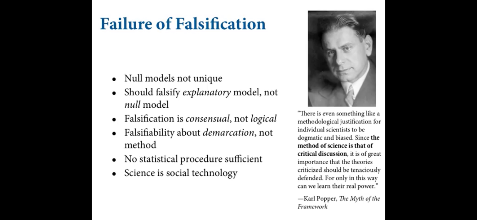**Paraphrasing from McElreath's lecture video:**Scientists have turned things upside down; originally the idea was that you had substantive of hypotheses that you would want to falsify and now we try to falsify silly null hypotheses that "nothing is going on". You should try to really build a hypothesis and test it not just reject that nothing is going on.> greatest obstacle that I encounter among students and colleagues is the tacit belief that the proper objective of statistical inference is to test null hypotheses> deductive falsification is impossible in nearly every scientific context::: {.callout-note collapse="true"}## Intricate argument for this, non-unique predictions of models> Many models correspond to the same hypothesis, and many hypotheses correspond to a single model. This makes strict falsification impossible. (2) Measurement matters. Even when we think the data falsify a model, another observer will debate our methods and measures. They don-t trust the data. Sometimes they are right.> All models are false, so what does it mean to falsify a model? One consequence of the requirement to work with models is that it's no longer possible to deduce that a hypothesis is false, just because we reject a model derived from it.> And so this fact yields a statistical model, MII, that predicts a power law in the data. In contrast the constant selection process model P1A predicts something quite different, MIII. Unfortunately, other selection models (P1B) imply the same statistical model, MII, as the neutral model. They also produce power laws> If we reject the null, we can't really conclude that selection matters, because there are other neutral models that predict different distributions of alleles. And if we fail to reject the null, we can't really conclude that evolution is neutral, because some selection models expect the same frequency distributionWhat about 'black swan' falsification?:> we most often face two simultaneous problems that make the swan fable misrepresentative. First, observations are prone to error, especially at the boundaries of scientific knowledge. Second, most hypotheses are quantitative, concerning degrees of existence, rather than discrete, concerning total presence or absence\H0 "Black swans are rare"Neutrinos case:> the "measurement" in this case is really an estimate from a statistical model, all false and true positives are possible..? usually measurement error is an issue. so black swan falsification is not so simple:::::: {.callout-note collapse="true"}## *Rethinking: Is NHST falsificationist?*Null hypothesis significance testing, NHST, is often identified with the falsificationist, or Popperian, philosophy of science. However, usually NHST is used to falsify a null hypothesis, not the actual research hypothesis. So the falsification is being done to something other than the explanatory model.:::::: {.callout-note collapse="true"}## DR question: What would a 'correct' falsificationist/hypothesis testing approach involve?I'm not sure I've actually ever seen the NHST or other 'falsificationist' framework defended or fully expounded. What are some good references for this?E.g., if we fail to reject a hypothesis, do we change our beliefs at all? What do we do with the evidence and data going forward?:::## We model...> attempting to mimic falsification is not a generally useful approach to statistical methods, what are we to do? We are to model.> Tools for golem engineering... We want to use our models for several distinct purposes: designing inquiry, extracting information from data, and making predictions. In this book I've chosen to focus on tools to help with each purpose. These tools are: (1) Bayesian data analysis (2) Model comparison (3) Multilevel models (4) Graphical causal models## Bayesian data analysis> Supposing you have some data, how should you use it to learn about the world? There is no uniquely correct answer to this question. Lots of approaches, both formal and heuristic, can be effective. But one of the most effective and general answers is to use Bayesian data analysis. Bayesian data analysis takes a question in the form of a model and uses logic to produce an answer in the form of probability distributions. In modest terms, Bayesian data analysis is no more than counting the numbers of ways the data could happen, according to our assumptions. Things that can happen more ways are more plausible.### Bayes vs frequentist probability> Bayesian probability ... includes as a special case another important approach, the frequentist approach. The frequentist approach requires that all probabilities be defined by connection to the frequencies of events in very large samples::: {.callout-note collapse="true"}## Frequentist: (DR question)> This leads to frequentist uncertainty being premised on imaginary resampling of data---if we were to repeat the measurement many many times, we would end up collecting a list of values that will have some pattern to it. It means also that parameters and models cannot have probability distributions, only measurements can. The distribution of these measurements is called a sampling distribution. This resampling is never done, and in general it doesn't even make sense---it is absurd to consider repeat sampling of the diversification of song birds in the Andes.DR_question: But Bayesian estimation also uses resampling. It also considers a draw from an imaginary distribution of 'true parameters'. This also seems absurd, so why is it better?> Bayesian golems treat "randomness" as a property of information, not of the world. We just use randomness to describe our uncertainty in the face of incomplete knowledge.Again, why is this better?:::::: {.callout-note collapse="true"}## Advantage of Bayesian approach? (DR question)> Note that the preceding description doesn't invoke anyone's "beliefs" or subjective opinions. Bayesian data analysis is just a logical procedure for processing information> Bayesian framework presents a distinct pedagogical advantage: many people find it more intuitive. Perhaps the best evidence for this is that very many scientists interpret non-Bayesian results in Bayesian terms, for example interpreting ordinary p-values as Bayesian posterior probabilities and non-Bayesian confidence intervals as Bayesian onesDR_question: how do we define a 'Bayesian CI'?:::### Model comparison and prediction.> Bayesian data analysis provides a way for models to learn from data. But when there is more than one plausible model-and in most mature fields there should be-how should we choose among them? One answer is to prefer models that make good predictions. This answer creates a lot of new questions, since knowing which model will make the best predictions seems to require knowing the future. We'll look at two related tools, neither of which knows the future: cross-validation and information criteria### Multilevel models> Multilevel models-also known as hierarchical, random effects, varying effects, or mixed effects models> Cross-validation and information criteria measure overfitting risk and help us to recognize it. Multilevel models actually do something about it. What they do is exploit an amazing trick known as partial poolinge.g., to... \>...adjust estimates for repeat sampling \> ... for imbalance in sampling... model variation explicitly (heterogeneity)::: {.callout-note collapse="true"}## DR question: Is multi-level modeling mainly about reducing overfitting?I had thought it was more about modeling the structure of the data in a more efficient way by reflecting something closer to the trye nature of randomness in the data. The 'regularization' (reducing overfit) seems to be a 'side benefit' of this. But is this a lucky coincidence and 'suspicious convergence'?:::> Multilevel models preserve the uncertainty in the original, pre-averaged values, while still using the average to make predictions> Suddenly single level models end up looking like mere components of multilevel models; multilevel regression deserves to be the default form of regression> even well-controlled treatments interact with unmeasured aspects of the individuals, groups, or populations studied### Graphical causal models> all we see is a statistical association. From the data alone, it could also be that the branches swaying makes the wind.::: {.callout-note collapse="true"}## A statistical model is an amazing association engine.> It makes it possible to detect associations between causes and their effects. But a statistical model is never sufficient for inferring cause, because the statistical model makes no distinction between the wind causing the branches to sway and the branches causing the wind to blow:::> ... a complete scientific model contains more information than a statistical model derived from it. And this additional information contains causal implications. These implications make it possible to test alternative causal models.::: {.callout-note collapse="true"}## Models that are causally incorrect can make better predictions than those that are causally correct> tools like cross-validation are very useful. But these tools will happily recommend models that contain confounding variables and suggest incorrect causal relationships. Why? Confounded relationships are real associations, and they can improve prediction. After all, if you look outside and see branches swaying, it really does predict wind.:::\**DAGs**> DAGs are heuristic---they are not detailed statistical models. But they allow us to deduce which statistical models can provide valid causal inferences, assuming the DAG is true. But where does a DAG itself come from? The terrible truth about statistical inference is that its validity relies upon information outside the data.\**Causal Salad**> the approach which dominates in many parts of biology and the social sciences is instead causal salad. Causal salad means tossing various 'control' variables into a statistical model, observing changes in estimates, and then telling a story about causation. Causal salad seems founded on the notion that only omitted variables can mislead us about causation. But included variables can just as easily confound us[^golem-4][^golem-4]: DR: See 'control strategies' in econometrics and their limitations. Adding a 'control' makes things worse, and formulas like the 'omitted variable bias' formula helps us understand this.> Instead of choosing among various black-box tools for testing null hypotheses, we should learn to build and analyze multiple non-null models of natural phenomena. To support this goal, the chapter introduced Bayesian inference, model comparison, multilevel models, and graphical causal models.## Session info {.unnumbered}```{r}sessionInfo()``````{r, echo = F, message = F, warning = F, results = "hide"}pacman::p_unload(pacman::p_loaded(), character.only =TRUE)ggplot2::theme_set(ggplot2::theme_grey())bayesplot::color_scheme_set("blue")```
