Transportation

Waterless transport

Prevalence

Only broodstock shrimp being transported by air and shrimp sold live are transported without water. Therefore, we think extensive farms are very unlikely to use waterless transportation, semi-intensive are somewhat likely, and intensive and super-intensive are very likely, though we are most uncertain about semi-intensive and intensive farms. We then weight these prevalences by the proportion of shrimp who are broodstock and the proportion that are sold live (which we estimate to be around 2%).

Not all broodstock are transported every year, some are found in domestic hatcheries, so we multiply the broodstock proportion by a distribution between 0.2 to 0.5 to account for this.

Our prevalence estimates are:

Extensive Semi-intensive Intensive Super-intensive
0–10% (mean 5%) 0–50% (mean 25%) 50–100% (mean 75%) 80–100% (mean 90%)
find_good_sd_binary(mean_val=0.05, tol=1e-6,
                   fifth_percentile=0, ninety_fifth_percentile=0.1)
find_good_sd_binary(mean_val=0.25, tol=1e-6,
                   fifth_percentile=0, ninety_fifth_percentile=0.5)
find_good_sd_binary(mean_val=0.75, tol=1e-6, 
                   fifth_percentile=0.5, ninety_fifth_percentile=1)
find_good_sd_binary(mean_val=0.9, tol=1e-6, 
                   fifth_percentile=0.8, ninety_fifth_percentile=1)
[1] 0.0368478
[1] 0.1727593
[1] 0.1725248
[1] 0.07310057

Sampling from beta distribution:

prev_nowater_stat <- data.frame(FarmType = c(
  "Extensive", "Semi-Intensive","Intensive","Super-Intensive"),
                               mean = c(0.05, 0.25, 0.75, 0.9),
                               sd = c(0.0368478, 0.1727593, 0.1725248, 0.07310057))
prev_nowater_dist<-mapply(sample_beta, prev_nowater_stat$mean, prev_nowater_stat$sd)
colnames(prev_nowater_dist)<-prev_nowater_stat$FarmType

prev_nowater_unadjusted<-as.data.frame(prev_nowater_dist)


sold_live<-runif(n, min=0.01, max=0.02)

broodstock_transported<-runif(n, min=0.2, max=0.5)

Waterless_Population_Proportion=((female_broodstock_prop*2)*broodstock_transported)+sold_live # adding shrimp who are sold live (estimated to be between 1% to 2% of shrimp) to proportion of broodstock (calculated as proportion of broodstock that are female, multiplied by two)
plot(density(Waterless_Population_Proportion))

prev_nowater<-prev_nowater_unadjusted*Waterless_Population_Proportion

Pain-Tracks

Our hypothesized pain category allocations are as follows:

dur_nowater = rtruncnorm(n, a=4, b=72, mean=30, sd = 8)

pain_nowater<-data.frame(sample_dirichlet(0.03, 0.06, 39, 60.91)) %>%
  `colnames<-`(paincategories)

Combine the intensity and duration information

paintrack_nowater<-(dur_nowater * pain_nowater)

We estimate a rough total shipment time as 15-35 hours. This is based on the fact that American Penaeid, Inc. report being three and a half hours away from international airports and that their customers are 8-28 hours away by plane. If we account for travel from the airport to the hatchery by assuming another 3.5 hours of travel time, then we arrive at our estimation of 15–35 hours. Our maximum duration comes from Benchmark Genetics Shrimp, who say they are prepared to acclimatize broodstock who have traveled for up to 72 hours.

Reducing temperature over 30 minutes in preparation for travel can causes oxidative stress, significantly increases mortality for trips of at least 10 hours (Xu et al., 2021). An operator we called at American Penaeid for our previous report estimated an ~85% survival rate for broodstock. Survival rates of “up to 80 percent” after 12 to 24 hours are often reported (Goodrick et al., 1993; Xu et al., 2021). Survival may actually be worse than is reported because conditions are likely better controlled in studies than they are in practice.

Weight the pain tracks by prevalence estimations and proportion of farming attributable to each farm type, as well as the average days lived by a shrimp.

nowater_farms<-data.frame(
  ext = paintrack_nowater*prev_nowater$Extensive*prop_sample$Ext,
  semi = paintrack_nowater*prev_nowater$`Semi-Intensive`*prop_sample$Semi,
  int = paintrack_nowater*prev_nowater$Intensive*prop_sample$Int,
  super = paintrack_nowater*prev_nowater$`Super-Intensive`*prop_sample$Super)

Add the pain categories across farm types and calculate the disabling-equivalent pain hours.

nowater<-nowater_farms %>%
  mutate(allfarms.Annoying = ext.Annoying + semi.Annoying + int.Annoying + super.Annoying,
         allfarms.Hurtful = ext.Hurtful + semi.Hurtful + int.Hurtful + super.Hurtful,
         allfarms.Disabling = ext.Disabling + semi.Disabling + int.Disabling + super.Disabling,
         allfarms.Excruciating = ext.Excruciating + semi.Excruciating + int.Excruciating + super.Excruciating,)

average_hours_nowater <- nowater %>%
  select(starts_with("allfarms"))

average_hours_nowater$Disabling_Equivalent<- (
  average_hours_nowater$allfarms.Annoying*Annoying_Weight) + (
    average_hours_nowater$allfarms.Hurtful*Hurtful_Weight) +(
      average_hours_nowater$allfarms.Disabling*Disabling_Weight)+(
        average_hours_nowater$allfarms.Excruciating*Excruciating_Weight)

nowater_summary<-cbind(round(rbind(
  (quantile(x =average_hours_nowater$allfarms.Annoying, probs = c(.05, .50, .95))), 
  (quantile(x =average_hours_nowater$allfarms.Hurtful, probs = c(.05, .50, .95))), 
  (quantile(x =average_hours_nowater$allfarms.Disabling, probs = c(.05, .50, .95))),
  (quantile(x =average_hours_nowater$allfarms.Excruciating, probs = c(.05, .50, .95))),
  (quantile(x =average_hours_nowater$Disabling_Equivalent, probs = c(.05, .50, .95)))), 10),
  "Mean" = colMeans(average_hours_nowater))
row.names(nowater_summary)<-c(
  "Annoying_nowater","Hurtful_nowater","Disabling_nowater", "Excruciating_nowater", "Disabling-Equivalent_Waterless_transport")
show_table(nowater_summary)
5% 50% 95% Mean
Annoying_nowater 0.0671463 0.1535126 0.2854261 0.1619378
Hurtful_nowater 0.0421207 0.0977142 0.1853087 0.1036312
Disabling_nowater 0.0000000 0.0000000 0.0008300 0.0001546
Excruciating_nowater 0.0000000 0.0000000 0.0002784 0.0000797
Disabling-Equivalent_Waterless_transport 0.0032081 0.0123728 0.1266984 0.0524292

Water-based transport

Prevalence

We do not assess brief cases of shrimp being transferred between tanks or ponds on the same farm—even though it is likely to cause some stress, the magnitude is not that of the other welfare threats we evaluate. Any shrimp transported between facilities within the same country are usually transported using water-based methods. Since most farms probably do not have on-site hatcheries, this means that most shrimp are transported in this way at some point, though we are somewhat uncertain about this. Super-intensive facilities are more likely to have on-site hatcheries.

Our prevalence estimates are:

Extensive Semi-intensive Intensive Super-intensive
50–100% (mean 75%) 90–100% (mean 95%) 50–90% (mean 70%) 10–90% (mean 50%)
find_good_sd_binary(mean_val=0.75, tol=1e-6,
                   fifth_percentile=0.5, ninety_fifth_percentile=1)
find_good_sd_binary(mean_val=0.95, tol=1e-6,
                   fifth_percentile=0.9, ninety_fifth_percentile=1)
find_good_sd_binary(mean_val=0.7, tol=1e-6, #sd_val=0.15,
                   fifth_percentile=0.5, ninety_fifth_percentile=0.9)
find_good_sd_binary(mean_val=0.5, tol=1e-6, #sd_val=0.05,
                   fifth_percentile=0.1, ninety_fifth_percentile=0.9)
[1] 0.1731566
[1] 0.0368054
[1] 0.1244102
[1] 0.2482915

Sampling from beta distribution:

prev_water_stat <- data.frame(FarmType = c(
  "Extensive", "Semi-Intensive","Intensive","Super-Intensive"),
                               mean = c(0.75, 0.95, 0.7, 0.5),
                               sd = c(0.1731566, 0.0368054, 0.1244102, 0.2482915))
prev_water_dist<-mapply(sample_beta, prev_water_stat$mean, prev_water_stat$sd)
colnames(prev_water_dist)<-prev_water_stat$FarmType

prev_water<-as.data.frame(prev_water_dist)

Pain-Tracks

Our hypothesized pain category allocations are as follows:

dur_water = rtruncnorm(n, a=0.1, b=72, mean=24, sd = 16)

pain_water<-data.frame(sample_dirichlet(0.03, 0.1, 25, 74.87)) %>%
  `colnames<-`(paincategories)

Combine the intensity and duration information

paintrack_water<-(dur_water * pain_water)

We estimate that water-based transport could, in theory, last from a few minutes up to 72 hours but that longer durations are less common.

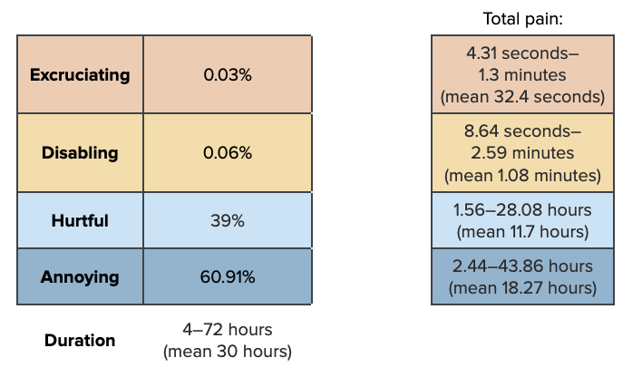
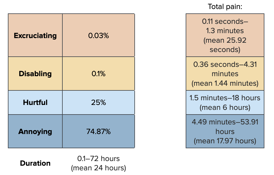
Mortality rates can reach 25% for 24-hour trips (Debnath et al., 2015, Table 3). High densities during transportation also pose risks to water quality, including dissolved oxygen depletion and increased ammonia concentrations. As some individuals become weaker, incidences of cannibalism can also rise. We account for these issues here because they are separate from dissolved oxygen and ammonia in farm ponds.

We assign pain to the ‘annoying’ and ‘hurtful’ categories to account for restricted movement and behavior, and to ‘disabling’ and ‘excruciating’ to account for cannibalism and mortality.

Then we combine all of the estimations for water-based transport.

water_farms<-data.frame(
  ext = paintrack_water*prev_water$Extensive*prop_sample$Ext,
  semi = paintrack_water*prev_water$`Semi-Intensive`*prop_sample$Semi,
  int = paintrack_water*prev_water$Intensive*prop_sample$Int,
  super = paintrack_water*prev_water$`Super-Intensive`*prop_sample$Super)

Add the pain categories across farm types and calculate the disabling-equivalent pain hours.

water<-water_farms %>%
  mutate(allfarms.Annoying = ext.Annoying + semi.Annoying + int.Annoying + super.Annoying,
         allfarms.Hurtful = ext.Hurtful + semi.Hurtful + int.Hurtful + super.Hurtful,
         allfarms.Disabling = ext.Disabling + semi.Disabling + int.Disabling + super.Disabling,
         allfarms.Excruciating = ext.Excruciating + semi.Excruciating + int.Excruciating + super.Excruciating,)

average_hours_water <- water %>%
  select(starts_with("allfarms"))

average_hours_water$Disabling_Equivalent<- (
  average_hours_water$allfarms.Annoying*Annoying_Weight) + (
    average_hours_water$allfarms.Hurtful*Hurtful_Weight) +(
      average_hours_water$allfarms.Disabling*Disabling_Weight)+(
        average_hours_water$allfarms.Excruciating*Excruciating_Weight)

water_summary<-cbind(round(rbind(
  (quantile(x =average_hours_water$allfarms.Annoying, probs = c(.05, .50, .95))), 
  (quantile(x =average_hours_water$allfarms.Hurtful, probs = c(.05, .50, .95))), 
  (quantile(x =average_hours_water$allfarms.Disabling, probs = c(.05, .50, .95))),
  (quantile(x =average_hours_water$allfarms.Excruciating, probs = c(.05, .50, .95))),
  (quantile(x =average_hours_water$Disabling_Equivalent, probs = c(.05, .50, .95)))), 10),
  "Mean" = colMeans(average_hours_water))
row.names(water_summary)<-c(
  "Annoying_water","Hurtful_water","Disabling_water", "Excruciating_water", "Disabling-Equivalent_Water-based_transport")
show_table(water_summary)
5% 50% 95% Mean
Annoying_water 2.6230708 13.9280642 29.1203058 14.6228313
Hurtful_water 0.8450727 4.5302856 10.1136136 4.8780652
Disabling_water 0.0000000 0.0000931 0.1064375 0.0195400
Excruciating_water 0.0000000 0.0000000 0.0190364 0.0058738
Disabling-Equivalent_Water-based_transport 0.0968607 0.6170167 8.4886314 3.5948063