prev_dens_stat <- data.frame(FarmType = c(
"Extensive", "Semi-Intensive","Intensive","Super-Intensive"),
mean = c(0.5, 0.8, 0.99, 0.99),
sd = c(0.1512446, 0.03808708, 0.001, 0.001))
prev_dens_dist<-mapply(sample_beta, prev_dens_stat$mean, prev_dens_stat$sd)
colnames(prev_dens_dist)<-prev_dens_stat$FarmType
prev_dens_dist[,3:4] <- 1
prev_dens<-as.data.frame(prev_dens_dist)Pond habitat
High density
To avoid double counting and because we assume most farmers using very high densities are using methods to prevent low DO and high ammonia, we are not counting the water-quality effects of high densities here.
We use observations by Rivera-Velázquez et al. (2008) and Medina-Reyna (2001) that shrimp in the wild are found at densities between 0.001 and 4.9 individuals per m2 as a reference value, assuming that this density range represents shrimp preferences.
We use the stocking densities from Table 3 of our main report to compare the wild shrimp densities with that of different farm types: - Extensive: ~<5 to 20 post-larvae per m2 - Semi-intensive: ~5 to 40 post-larvae per m2 - Intensive: ~40 to 130 post-larvae per m2 - Super-intensive: ~130 to >300 post-larvae per m2
Prevalence
Stocking density increases with increasing farm intensity.
Extensive farms use low densities but may still have shrimp at somewhat higher levels than their wild counterparts. We think intensive and super-intensive farms are definitely using high densities, since it is a defining feature of these farm types.
Our estimates are:
| Extensive | Semi-intensive | Intensive | Super-intensive |
|---|---|---|---|
| 25–75% (mean 50%) | 75–100% (mean 80%) | 100% | 100% |
find_good_sd_binary(mean_val=0.5, tol=1e-6,
                   fifth_percentile=0.25, ninety_fifth_percentile=0.75)
find_good_sd_binary(mean_val=0.8, tol=1e-6,
                   fifth_percentile=0.75, ninety_fifth_percentile=1)
[1] 0.1512446[1] 0.03808708Sampling from beta distribution:
Pain-Tracks
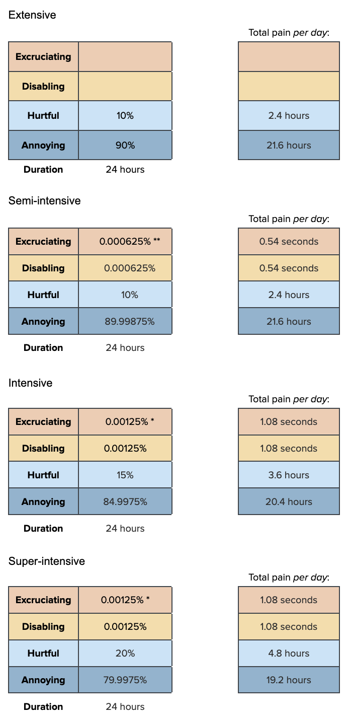
Percentages marked with * assume death from cannibalism happens roughly every four weeks and causes one minute of excruciating and disabling pain together when it does happen.
Percentage marked with ** assumes death from cannibalism happens once every eight weeks and causes one minute of excruciating and disabling pain together when it does happen.
dur_dens_ext<-24
dur_dens_semi<-24
dur_dens_int<-24
dur_dens_super<-24

pain_dens_ext<-data.frame(
  Excruciating = 0,
  Disabling = 0) %>%
  cbind(sample_dirichlet(0, 0, 10, 90)) %>%
  `colnames<-`(paincategories)

pain_dens_semi<-data.frame(sample_dirichlet(0.000625, 0.000625, 10, 89.99875)) %>%
  `colnames<-`(paincategories)

pain_dens_int<-data.frame(sample_dirichlet(0.00125, 0.00125, 15, 84.9975)) %>%
  `colnames<-`(paincategories)

pain_dens_super<-data.frame(sample_dirichlet(0.00125, 0.00125, 20, 79.9975)) %>%
  `colnames<-`(paincategories)
Combine the intensity and duration information
paintrack_dens_ext<-(dur_dens_ext * pain_dens_ext)

paintrack_dens_semi<-(dur_dens_semi * pain_dens_semi)

paintrack_dens_int<-(dur_dens_int * pain_dens_int)

paintrack_dens_super<-(dur_dens_super * pain_dens_super)Weight the pain tracks by prevalence estimations and proportion of farming attributable to each farm type, as well as the average days lived by a shrimp.
dens_farms<-data.frame(
  ext = paintrack_dens_ext*prev_dens$Extensive*prop_sample$Ext*average_days_lived,
  semi = paintrack_dens_semi*prev_dens$`Semi-Intensive`*prop_sample$Semi*average_days_lived,
  int = paintrack_dens_int*prev_dens$Intensive*prop_sample$Int*average_days_lived,
  super = paintrack_dens_super*prev_dens$`Super-Intensive`*prop_sample$Super*average_days_lived)
Add the pain categories across farm types and calculate the disabling-equivalent pain hours.
dens<-dens_farms %>%
  mutate(allfarms.Annoying = ext.Annoying + semi.Annoying + int.Annoying + super.Annoying,
         allfarms.Hurtful = ext.Hurtful + semi.Hurtful + int.Hurtful + super.Hurtful,
         allfarms.Disabling = ext.Disabling + semi.Disabling + int.Disabling + super.Disabling,
         allfarms.Excruciating = ext.Excruciating + semi.Excruciating + int.Excruciating + super.Excruciating,)

average_hours_dens <- dens %>%
  select(starts_with("allfarms"))

average_hours_dens$Disabling_Equivalent<- (
  average_hours_dens$allfarms.Annoying*Annoying_Weight) + (
    average_hours_dens$allfarms.Hurtful*Hurtful_Weight) +(
      average_hours_dens$allfarms.Disabling*Disabling_Weight)+(
        average_hours_dens$allfarms.Excruciating*Excruciating_Weight)

density_summary<-cbind(round(rbind(
  (quantile(x =average_hours_dens$allfarms.Annoying, probs = c(.05, .50, .95))),
  (quantile(x =average_hours_dens$allfarms.Hurtful, probs = c(.05, .50, .95))),
  (quantile(x =average_hours_dens$allfarms.Disabling, probs = c(.05, .50, .95))),
  (quantile(x =average_hours_dens$allfarms.Excruciating, probs = c(.05, .50, .95))),
  (quantile(x =average_hours_dens$Disabling_Equivalent, probs = c(.05, .50, .95)))), 10),
  "Mean" = colMeans(average_hours_dens))
row.names(density_summary)<-c(
  "Annoying_dens","Hurtful_dens","Disabling_dens", "Excruciating_dens", "Disabling-Equivalent_High_stocking_density")
show_table(density_summary)| 5% | 50% | 95% | Mean | |
|---|---|---|---|---|
| Annoying_dens | 260.567270 | 2493.46325 | 3321.0275534 | 2160.2088110 |
| Hurtful_dens | 40.660056 | 377.53420 | 617.3710350 | 351.8301888 |
| Disabling_dens | 0.000000 | 0.00000 | 0.0000001 | 0.0272782 |
| Excruciating_dens | 0.000000 | 0.00000 | 0.0000000 | 0.0265697 |
| Disabling-Equivalent_High_stocking_density | 5.234926 | 49.02643 | 112.2994853 | 63.7122589 |
Lack of substrate
Here, we are considering both a lack of natural, burrowable substrate and a lack of artificial structures the shrimp can climb or cling to.
Prevalence
Earthen ponds, typically used for extensive and sometimes semi-intensive ponds likely have a burrowable substrate on the pond bottom. Some semi-intensive ponds are lined with plastic, however. Intensive and super-intensive ponds are plastic or concrete lined, or are raised tanks, which would not have substrate available to shrimp.
95% of semi-intensive farms in SWP’s India Scoping Report and the one intensive farm interviewed, said they had substrate where shrimps can bury themselves.
Using artificial screens or other structures shrimp can cling to is not standard practice in any farm type. It is possible that extensive and some semi-intensive ponds may have plants growing in them, which shrimp could use for this purpose, though we are very uncertain about this.
Our prevalence estimates are:
| Extensive | Semi-intensive | Intensive | Super-intensive |
|---|---|---|---|
| 0–15% (mean 5%) | 25–75% (mean 50%) | 90–100% (mean 95%) | 100% |
find_good_sd_binary(mean_val=0.05, tol=1e-6,
                   fifth_percentile=0, ninety_fifth_percentile=0.15)
find_good_sd_binary(mean_val=0.5, tol=1e-6,
                   fifth_percentile=0.25, ninety_fifth_percentile=0.75)
find_good_sd_binary(mean_val=0.95, tol=1e-6, #sd_val=0.15,
                   fifth_percentile=0.9, ninety_fifth_percentile=1)
[1] 0.07970699[1] 0.1513085[1] 0.03695588Sampling from beta distribution:
prev_subst_stat <- data.frame(FarmType = c(
  "Extensive", "Semi-Intensive","Intensive","Super-Intensive"),
                               mean = c(0.05, 0.5, 0.95, 0.99),
                               sd = c(0.07970699, 0.1513085, 0.03695588, 0.001))
prev_subst_dist<-mapply(sample_beta, prev_subst_stat$mean, prev_subst_stat$sd)
colnames(prev_subst_dist)<-prev_subst_stat$FarmType
prev_subst_dist[,4]<-1

prev_subst<-as.data.frame(prev_subst_dist)
Pain-Tracks
Where no substrate is present, shrimp in different farming systems are likely to have the same experience so we do one pain track for all farm types. However, P. monodon burrow more than P. vannamei so we do species-specific pain-tracks, one for P. vannamei and other penaeids and one for P. monodon, then weight by the proportion of farmed shrimp that are that species or group. P. monodon would usually burrow for around half the day in the wild.
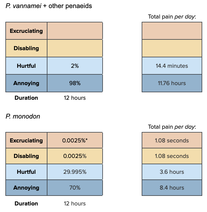
Durations marked * assume death from cannibalism happens once every four weeks and causes one minute of excruciating and disabling pain together when it does.
dur_subst<-12

pain_subst_vannamei<-data.frame(
  Excruciating = 0,
  Disabling = 0) %>%
  cbind(sample_dirichlet(0, 0, 2, 98)) %>%
  `colnames<-`(paincategories)

pain_subst_monodon<-data.frame(sample_dirichlet(0.0025, 0.0025, 29.995, 70)) %>%
  `colnames<-`(paincategories)
Combine the intensity and duration information and weight by the proportion of farmed shrimp that are that species or group.
paintrack_subst_vannamei<-(dur_subst * pain_subst_vannamei * (prop_allspecies_dof$van_prop+prop_allspecies_dof$otherpen_prop))

paintrack_subst_monodon<-(dur_subst * pain_subst_monodon * prop_allspecies_dof$mon_prop)Weight the pain tracks by prevalence estimations and proportion of farming attributable to each farm type, as well as the average days lived by a shrimp.
subst_farms<-data.frame(
  ext = (paintrack_subst_vannamei+paintrack_subst_monodon)*prev_subst$Extensive*prop_sample$Ext*average_days_lived,
  semi = (paintrack_subst_vannamei+paintrack_subst_monodon)*prev_subst$`Semi-Intensive`*prop_sample$Semi*average_days_lived,
  int = (paintrack_subst_vannamei+paintrack_subst_monodon)*prev_subst$Intensive*prop_sample$Int*average_days_lived,
  super = (paintrack_subst_vannamei+paintrack_subst_monodon)*prev_subst$`Super-Intensive`*prop_sample$Super*average_days_lived)
Add the pain categories across farm types and calculate the disabling-equivalent pain hours.
subst<-subst_farms %>%
  mutate(allfarms.Annoying = ext.Annoying + semi.Annoying + int.Annoying + super.Annoying,
         allfarms.Hurtful = ext.Hurtful + semi.Hurtful + int.Hurtful + super.Hurtful,
         allfarms.Disabling = ext.Disabling + semi.Disabling + int.Disabling + super.Disabling,
         allfarms.Excruciating = ext.Excruciating + semi.Excruciating + int.Excruciating + super.Excruciating,)

average_hours_subst <- subst %>%
  select(starts_with("allfarms"))

average_hours_subst$Disabling_Equivalent<- (
  average_hours_subst$allfarms.Annoying*Annoying_Weight) + (
    average_hours_subst$allfarms.Hurtful*Hurtful_Weight) +(
      average_hours_subst$allfarms.Disabling*Disabling_Weight)+(
        average_hours_subst$allfarms.Excruciating*Excruciating_Weight)

subst_summary<-cbind(round(rbind(
  (quantile(x =average_hours_subst$allfarms.Annoying, probs = c(.05, .50, .95))),
  (quantile(x =average_hours_subst$allfarms.Hurtful, probs = c(.05, .50, .95))),
  (quantile(x =average_hours_subst$allfarms.Disabling, probs = c(.05, .50, .95))),
  (quantile(x =average_hours_subst$allfarms.Excruciating, probs = c(.05, .50, .95))),
  (quantile(x =average_hours_subst$Disabling_Equivalent, probs = c(.05, .50, .95)))), 10),
  "Mean" = colMeans(average_hours_subst))
row.names(subst_summary)<-c(
  "Annoying_subst","Hurtful_subst","Disabling_subst", "Excruciating_subst", "Disabling-Equivalent_Lack_of_substrate")
show_table(subst_summary)| 5% | 50% | 95% | Mean | |
|---|---|---|---|---|
| Annoying_subst | 123.312084 | 1175.07878 | 1591.68529 | 1023.9393168 |
| Hurtful_subst | 4.645325 | 43.47604 | 97.39193 | 45.7305333 |
| Disabling_subst | 0.000000 | 0.00000 | 0.00000 | 0.0020288 |
| Excruciating_subst | 0.000000 | 0.00000 | 0.00000 | 0.0021100 |
| Disabling-Equivalent_Lack_of_substrate | 1.227130 | 11.47259 | 24.15215 | 12.5632945 |
Predators
Prevalence
We were unable to find estimates of the incidence of predators or data on how much mortality predators typically cause. However, a consulted expert suggested that predators are usually well-managed in current shrimp farming practices. We expect that where this issue is present, it is usually in extensive farms.
We give super-intensive farms a value of zero because super-intensive are indoor, closed, predator-free systems.
Our prevalence estimates are:
| Extensive | Semi-intensive | Intensive | Super-intensive |
|---|---|---|---|
| 0–50% (mean 25%) | 0–30% (mean 15%) | 0–10% (mean 5%) | 0% |
find_good_sd_binary(mean_val=0.25, tol=1e-6,
                   fifth_percentile=0, ninety_fifth_percentile=0.5)
find_good_sd_binary(mean_val=0.15, tol=1e-6,
                   fifth_percentile=0, ninety_fifth_percentile=0.3)
find_good_sd_binary(mean_val=0.05, tol=1e-6, #sd_val=0.15,
                   fifth_percentile=0, ninety_fifth_percentile=0.1)
[1] 0.17334[1] 0.1077494[1] 0.03673223Sampling from beta distribution:
prev_pred_stat <- data.frame(FarmType = c(
  "Extensive", "Semi-Intensive","Intensive","Super-Intensive"),
                               mean = c(0.25, 0.15, 0.05, 0.001),
                               sd = c(0.17334, 0.1077494, 0.03673223, 0.001))
prev_pred_dist<-mapply(sample_beta, prev_pred_stat$mean, prev_pred_stat$sd)
colnames(prev_pred_dist)<-prev_pred_stat$FarmType
prev_pred_dist[,4]<-0

prev_pred<-as.data.frame(prev_pred_dist)
Pain-Tracks
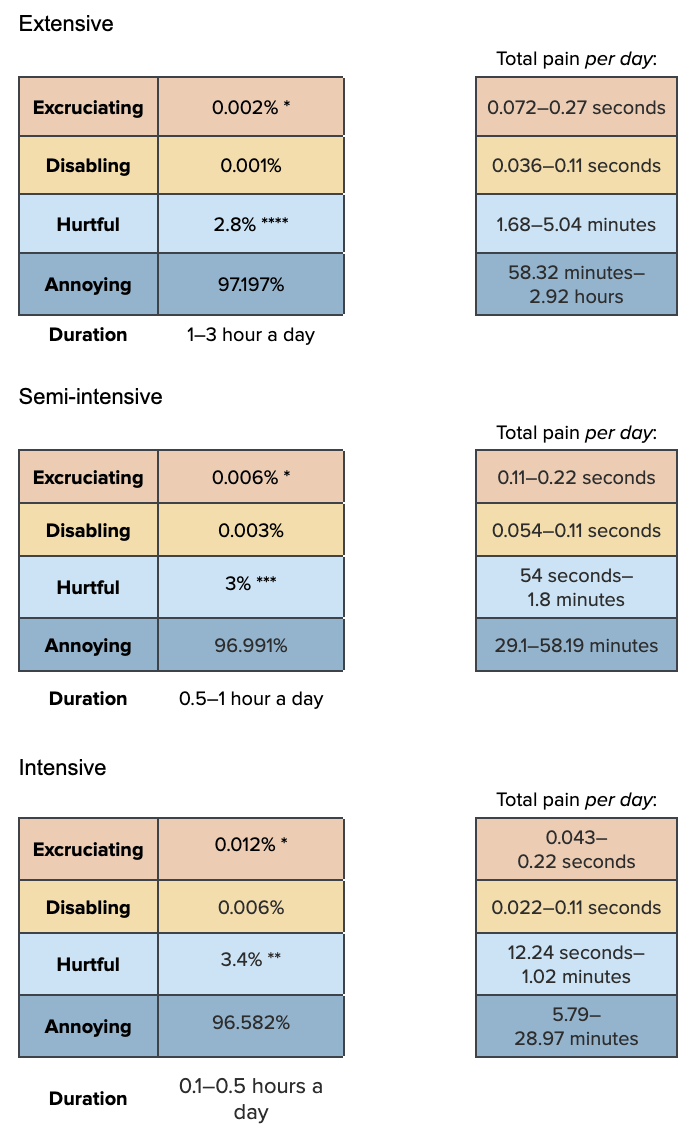
Durations marked * assume 10 seconds of excruciating pain (at the longest duration) if a shrimp is eaten by a predator, and that one in every 50 shrimp is eaten
Durations marked ** assume one minute of high predator vigilance (i.e. ceasing some activities they would otherwise do) a day at the longest duration – shrimp are likely not vigilant to birds very much if the water turbidity is high, but they are a prey species so likely exhibit predator vigilance and avoidance, so we start with an estimate of a minute a day
Those marked *** assume two minutes of high predator vigilance a day at the longest duration, hypothesizing that vigilance increases the longer predators are present
Those marked **** assume 5 minutes of high predator vigilance a day at the longest duration.
dur_pred_ext<-runif(n, 1, 3)
dur_pred_semi<-runif(n, 0.5, 1)
dur_pred_int<-runif(n, 0.1, 0.5)
dur_pred_super<-runif(n, 0, 0)

pain_pred_ext<-data.frame(sample_dirichlet(0.002, 0.001, 2.8, 97.197)) %>%
  `colnames<-`(paincategories)

pain_pred_semi<-data.frame(sample_dirichlet(0.006, 0.003, 3, 96.991)) %>%
  `colnames<-`(paincategories)

pain_pred_int<-data.frame(sample_dirichlet(0.012, 0.006, 3.4, 96.582)) %>%
  `colnames<-`(paincategories)

pain_pred_super<-data.frame(
  Excruciating = 0,
  Disabling = 0,
  Hurtful = 0,
  Annoying = 0) %>%
  `colnames<-`(paincategories)
Combine the intensity and duration information
paintrack_pred_ext<-(dur_pred_ext * pain_pred_ext)

paintrack_pred_semi<-(dur_pred_semi * pain_pred_semi)

paintrack_pred_int<-(dur_pred_int * pain_pred_int)

paintrack_pred_super<-(dur_pred_super * pain_pred_super)pred_farms<-data.frame(
ext = paintrack_pred_ext*prev_pred$Extensive*prop_sample$Ext*average_days_lived,
semi = paintrack_pred_semi*prev_pred$`Semi-Intensive`*prop_sample$Semi*average_days_lived,
int = paintrack_pred_int*prev_pred$Intensive*prop_sample$Int*average_days_lived,
super = paintrack_pred_super*prev_pred$`Super-Intensive`*prop_sample$Super*average_days_lived)Add the pain categories across farm types and calculate the disabling-equivalent pain hours.
pred<-pred_farms %>%
  mutate(allfarms.Annoying = ext.Annoying + semi.Annoying + int.Annoying + super.Annoying,
         allfarms.Hurtful = ext.Hurtful + semi.Hurtful + int.Hurtful + super.Hurtful,
         allfarms.Disabling = ext.Disabling + semi.Disabling + int.Disabling + super.Disabling,
         allfarms.Excruciating = ext.Excruciating + semi.Excruciating + int.Excruciating + super.Excruciating,)

average_hours_pred <- pred %>%
  select(starts_with("allfarms"))

average_hours_pred$Disabling_Equivalent<- (
  average_hours_pred$allfarms.Annoying*Annoying_Weight) + (
    average_hours_pred$allfarms.Hurtful*Hurtful_Weight) +(
      average_hours_pred$allfarms.Disabling*Disabling_Weight)+(
        average_hours_pred$allfarms.Excruciating*Excruciating_Weight)

pred_summary<-cbind(round(rbind(
  (quantile(x =average_hours_pred$allfarms.Annoying, probs = c(.05, .50, .95))),
  (quantile(x =average_hours_pred$allfarms.Hurtful, probs = c(.05, .50, .95))),
  (quantile(x =average_hours_pred$allfarms.Disabling, probs = c(.05, .50, .95))),
  (quantile(x =average_hours_pred$allfarms.Excruciating, probs = c(.05, .50, .95))),
  (quantile(x =average_hours_pred$Disabling_Equivalent, probs = c(.05, .50, .95)))), 10),
  "Mean" = colMeans(average_hours_pred))
row.names(pred_summary)<-c(
  "Annoying_pred","Hurtful_pred","Disabling_pred", "Excruciating_pred", "Disabling-Equivalent_Predators")
show_table(pred_summary)| 5% | 50% | 95% | Mean | |
|---|---|---|---|---|
| Annoying_pred | 0.8050590 | 7.9419517 | 24.0954781 | 9.4924930 |
| Hurtful_pred | 0.0209389 | 0.2115089 | 0.8025060 | 0.2849289 |
| Disabling_pred | 0.0000000 | 0.0000000 | 0.0000306 | 0.0001923 |
| Excruciating_pred | 0.0000000 | 0.0000000 | 0.0005100 | 0.0003953 |
| Disabling-Equivalent_Predators | 0.0072090 | 0.0748735 | 0.4028101 | 0.2846178 |