1 Survival curves model

The aim of this chapter is to model the pre-slaughter mortality rates of farmed shrimp across the production cycle. We use the Guesstimate model by Waldhorn and Autric (2023), in which they estimated the number of shrimp farmed annually and alive at any time, to form the basis of our model.

We focus on three taxa: P. vannamei, P. monodon, and Macrobrachium—the latter covers M. rosenbergii and M. nipponese.

First, load the required packages and set the seed so that our data is reproducible.

library(dplyr)
library(tidyr)
library(janitor)
library(kde1d)
library(kableExtra)
library(survival)
library(ggsurvfit)
library(ggpubr)
library(patchwork)


# at time of publication we need the ggplot v3.4.4 because the most recent version (3.5.0) does not work with the patchwork package
old.version <- "http://cran.r-project.org/src/contrib/Archive/ggplot2/ggplot2_3.4.4.tar.gz"
install.packages(old.version, repos=NULL, type="source")

library(ggplot2)

set.seed(123)

Next, create functions to compare the summary statistics of two data frames.

give.summary=function(x,y){
knitr::kable(data.frame("original"=c(quantile(x, probs=c(0.05,0.5,0.95)),
    mean=mean(x), sd=sd(x), min=min(x), max=max(x)),
    "new"=c(quantile(y, probs=c(0.05,0.5,0.95)),
    mean=mean(y), sd=sd(y), min=min(y), max=max(y))), table.attr = 'data-quarto-disable-processing="true"') %>%
    kable_styling(full_width=FALSE, font_size=9) 
}

give.full.summary=function(a1, b1, c1, a2, b2, c2){
  knitr::kable(data.frame(
    "original"=c(quantile(a1, probs=c(0.05,0.5,0.95)),
    mean=mean(a1), sd=sd(a1), min=min(a1), max=max(a1)),
    "new"=c(quantile(a2, probs=c(0.05,0.5,0.95)),
    mean=mean(a2), sd=sd(a2), min=min(a2), max=max(a2)),
    "original"=c(quantile(b1, probs=c(0.05,0.5,0.95)),
    mean=mean(b1), sd=sd(b1), min=min(b1), max=max(b1)),
    "new"=c(quantile(b2, probs=c(0.05,0.5,0.95)),
    mean=mean(b2), sd=sd(b2), min=min(b2), max=max(b2)),
    "original"=c(quantile(c1, probs=c(0.05,0.5,0.95)),
    mean=mean(c1), sd=sd(c1), min=min(c1), max=max(c1)),
    "new"=c(quantile(c2, probs=c(0.05,0.5,0.95)),
    mean=mean(c2), sd=sd(c2), min=min(c2), max=max(c2))),
    table.attr = 'data-quarto-disable-processing="true"',
    col.names = rep(c("original", "new"), 3)) %>%
    kable_styling(full_width=FALSE, font_size=9)
}

1.1 Preparing data

For all the .csv files used in this chapter, see the GitHub repository.

We downloaded the 5000 samples created by the Guesstimate model for the three taxa for each of:

The number of individuals that die on farms annually
Days lived by life stage, given the shrimp dies in the life stage (e.g., a shrimp that dies in the larval stage lives for an average of two days)
Mortality rates within each life stage, conditional upon having lived to that life stage

Note: the guesstimate model re-samples each time it is opened so the figures you see may differ slightly from those used here.

To best sample from the Guesstimate data (especially the tails of the distributions) and to remove errors created by Guesstimate (e.g., negative values), we generated 100,000 synthetic samples for each of these, based off the original 5000 guesstimate samples. To do this, we use the kde1d function, which estimates a kernel density function from the 5000 samples, and the rkde1d function, which generates n (in our case 100,000) samples from the estimated kernel density.

1.1.1 Number of shrimp that die on farms annually

Starting with the number of individuals that die on farms annually, we first load the samples from Guesstimate, then make the 100,000 samples.

# loading die on farms samples, taken from Guesstimate model

allspecies_dof_samp<-read.csv("../data/guesstimate/die_on_farm_samples.csv", header=TRUE, sep=",")

vannamei_dof<-allspecies_dof_samp$vannamei[allspecies_dof_samp$vannamei>0] %>% # Cell GZ in the Guesstimate model
  # removing negative values created by Guesstimate
  kde1d(xmin=0) %>% # running kde1d function and ensuring no values below 0 are created
  rkde1d(100000,.) # creating 100,000 samples from the data

# now we can compare the summary statistics of the old and new data
give.summary(allspecies_dof_samp$vannamei, vannamei_dof)%>%
  add_header_above(c("P. vannamei"=3)) # creating a header that spans the full 3 columns of the table
# repeat this for other taxa

monodon_dof<-allspecies_dof_samp$monodon[allspecies_dof_samp$monodon>0] %>% # Cell ES in the Guesstimate model
  kde1d(xmin=0) %>%
  rkde1d(100000,.)
give.summary(allspecies_dof_samp$monodon, monodon_dof)%>%
  add_header_above(c("P. monodon"=3))
macro_dof<-allspecies_dof_samp$macrobrachium[allspecies_dof_samp$macrobrachium>0] %>% # Cell BZ in the Guesstimate model
  kde1d(xmin=0) %>%
  rkde1d(100000,.)
give.summary(allspecies_dof_samp$macrobrachium, macro_dof) %>%
  add_header_above(c("Macrobrachium"=3))

P. vannamei
	original	new
5%	3.539500e+11	3.517307e+11
50%	5.810000e+11	5.791339e+11
95%	9.980500e+11	1.003184e+12
mean	6.192688e+11	6.234259e+11
sd	4.229737e+11	2.956778e+11
min	-1.490000e+13	5.696191e+08
max	8.250000e+12	8.060032e+12

P. monodon
	original	new
5%	29395000000	29124727717
50%	52900000000	52723011534
95%	93605000000	93893586229
mean	56130860000	56014290871
sd	20685345595	20640193828
min	16000000000	21079491
max	216000000000	215982898786

Macrobrachium
	original	new
5%	9.400000e+10	9.381296e+10
50%	1.650000e+11	1.646129e+11
95%	3.180000e+11	3.190560e+11
mean	1.802238e+11	1.804668e+11
sd	8.362092e+10	8.210190e+10
min	4.660000e+10	3.012260e+08
max	1.620000e+12	1.604432e+12

Now we can calculate the proportion of farmed shrimp accounted for by each species for each of our 100,000 samples.

allspecies_dof<-cbind(vannamei_dof, monodon_dof, macro_dof) # combining the 100,000 samples for each species into a data frame

prop_allspecies<-as.data.frame(allspecies_dof) %>% 
  rowwise() %>%
  mutate(van_prop=vannamei_dof/sum(vannamei_dof, monodon_dof, macro_dof), # calculating each sample as a proportion of the total shrimp, row-wise
         mon_prop=monodon_dof/sum(vannamei_dof, monodon_dof, macro_dof),
         macro_prop=macro_dof/sum(vannamei_dof, monodon_dof, macro_dof))

prop_allspecies_dof<-as.data.frame(prop_allspecies[,4:6]) # keeping only the proportions

1.1.2 Days lived by life stage

Next we load the data for the number of days lived by a shrimp, given that it dies within a certain life stage. The four life stages are larval, postlarval, juvenile-adult, and (if a shrimp survives all three) the days lived before slaughter, which we call the total farmed days.

# First load the data
vannamei_days_samp<-read.csv("../data/guesstimate/vannamei_days_lived.csv", header=TRUE,sep=",") # Cells TE, VO, XM, and QV in the Guesstimate model
monodon_days_samp<-read.csv("../data/guesstimate/monodon_days_lived.csv", header=TRUE, sep=",") # Cells MF, HI, OZ, and LW in the Guesstimate model
macrobrachium_days_samp<-read.csv("../data/guesstimate/macrobrachium_days_lived.csv", header=TRUE, sep=",") # Cells AS, BJ, EY, and XT in the Guesstimate model

# Next make the 100,000 samples
vannamei_days_lived<-data.frame(larval=rep(NA, 100000), # create empty data frame
                                postlarval=rep(NA, 100000),
                                juvenile.adult=rep(NA, 100000),
                                total.farmed=rep(NA, 100000))

# fill empty data frame with data simulated from Guesstimate data using kde1d function
vannamei_days_lived$larval<-vannamei_days_samp$larval %>% 
  kde1d(xmin=0) %>% # shrimp can't live for fewer than 0 days so we limit the distribution
  rkde1d(100000,.)
vannamei_days_lived$postlarval<-vannamei_days_samp$postlarval %>% 
  kde1d() %>%
  rkde1d(100000,.)
vannamei_days_lived$juvenile.adult<-vannamei_days_samp$juvenile.adult %>% 
  kde1d() %>%
  rkde1d(100000,.)

give.full.summary(vannamei_days_samp$larval,
                  vannamei_days_samp$postlarval,
                  vannamei_days_samp$juvenile.adult,
                  vannamei_days_lived$larval,
                  vannamei_days_lived$postlarval,
                  vannamei_days_lived$juvenile.adult) %>%
  add_header_above(c(" "=1, "larval" = 2, "postlarval" = 2, "juvenile-subadult" = 2)) %>%
  add_header_above(c("P. vannamei"=7))
# repeat for other species
monodon_days_lived<-data.frame(larval=rep(NA, 100000),
                               postlarval=rep(NA, 100000),
                               juvenile.adult=rep(NA, 100000),
                               total.farmed=rep(NA, 100000))

monodon_days_lived$larval<-monodon_days_samp$larval %>% 
  kde1d(xmin=0) %>% # shrimp can't live for fewer than 0 days so we limit the distribution
  rkde1d(100000,.)
monodon_days_lived$postlarval<-monodon_days_samp$postlarval %>% 
  kde1d() %>%
  rkde1d(100000,.)
monodon_days_lived$juvenile.adult<-monodon_days_samp$juvenile.adult %>% 
  kde1d() %>%
  rkde1d(100000,.)

give.full.summary(monodon_days_samp$larval,
                  monodon_days_samp$postlarval,
                  monodon_days_samp$juvenile.adult,
                  monodon_days_lived$larval,
                  monodon_days_lived$postlarval,
                  monodon_days_lived$juvenile.adult) %>%
  add_header_above(c(" "=1, "larval" = 2, "postlarval" = 2, "juvenile-subadult" = 2)) %>%
  add_header_above(c("P. monodon"=7))
macro_days_lived<-data.frame(larval=rep(NA, 100000), 
                             postlarval=rep(NA, 100000),
                             juvenile.adult=rep(NA, 100000),
                             total.farmed=rep(NA, 100000))

macro_days_lived$larval<-macrobrachium_days_samp$larval %>% 
  kde1d(xmin=0) %>% # shrimp can't live for fewer than 0 days so we limit the distribution 
  rkde1d(100000,.)
macro_days_lived$postlarval<-macrobrachium_days_samp$postlarval %>% 
  kde1d() %>%
  rkde1d(100000,.)
macro_days_lived$juvenile.adult<-macrobrachium_days_samp$juvenile.adult %>% 
  kde1d() %>%
  rkde1d(100000,.)

give.full.summary(macrobrachium_days_samp$larval,
                  macrobrachium_days_samp$postlarval,
                  macrobrachium_days_samp$juvenile.adult,
                  macro_days_lived$larval,
                  macro_days_lived$postlarval,
                  macro_days_lived$juvenile.adult) %>%
  add_header_above(c(" "=1, "larval" = 2, "postlarval" = 2, "juvenile-subadult" = 2)) %>%
  add_header_above(c("Macrobrachium"=7))

P. vannamei
	larval		postlarval		juvenile-subadult
	original	new	original	new	original	new
5%	0.5023743	0.4902677	11.154996	11.154865	53.13992	54.03571
50%	2.1023025	2.1120241	14.918215	14.957922	80.29052	80.32173
95%	8.5356682	8.9065270	20.017363	20.061194	106.91953	106.09696
mean	3.1018999	3.0744436	15.171321	15.198329	80.38564	80.26579
sd	3.2349854	3.1241976	2.734755	2.732966	17.21552	16.85421
min	0.1249571	0.0002519	7.741822	7.395876	50.03272	44.74333
max	33.8854679	33.7981077	30.754078	31.837442	109.99987	115.53883

P. monodon
	larval		postlarval		juvenile-subadult
	original	new	original	new	original	new
5%	0.4963115	0.4996946	11.001184	11.068435	34.93126	35.489895
50%	2.2152736	2.1858878	16.571929	16.617385	70.11952	70.076832
95%	9.6407133	9.5278613	25.015574	24.962607	136.61865	136.631247
mean	3.2634577	3.2441306	17.106562	17.157913	76.12007	76.350636
sd	3.6398201	3.4359323	4.356787	4.337294	33.43386	33.148128
min	0.0212167	0.0009423	6.723713	5.253515	13.39687	2.849361
max	96.7623124	68.5132450	44.915889	46.008715	337.47740	338.425447

Macrobrachium
	larval		postlarval		juvenile-subadult
	original	new	original	new	original	new
5%	1.9786751	1.9602180	29.987507	30.20970	60.63581	61.08796
50%	7.6767357	7.6056272	42.342525	42.52669	95.11617	95.69554
95%	29.9404670	29.3428149	59.741628	59.89201	149.64495	150.46335
mean	10.6956641	10.6289836	43.351758	43.47981	98.96567	99.29394
sd	10.5057846	10.1343738	9.262974	9.20008	27.81269	27.65936
min	0.4628982	0.0007937	20.471376	17.33767	31.35562	23.32129
max	159.2862181	155.5098833	82.711654	85.97558	300.38509	301.48431

Guesstimate produced a few large numbers of over one year for the total days farmed, which seems incorrect, so we remove these and restrict to:

215 days for P. vannamei (FAO (2009a) suggests the maximum cycle is 6 months in ongrowing with around a month of development prior to that, 7 months = ~214 days)
245 days for P. monodon (FAO (2009b) suggests the maximum cycle is >6 months in ongrowing, so we assume ~7 months, with around a month of development prior to that, 8 months = ~244 days)
335 day for Macrobrachium (New (2010, p.22; p.129) suggests that 11 months is the typical maximum length of a production cycle, 11 months= ~335.5 days)

The kde1d function will still produce a few samples just above this estimation.

vannamei_days_lived_total<-vannamei_days_samp$total_farmed_d[vannamei_days_samp$total_farmed_d<215]
vannamei_days_lived$total.farmed<-vannamei_days_lived_total %>% 
  kde1d() %>% 
  rkde1d(100000,.)
give.summary(vannamei_days_lived_total, vannamei_days_lived$total.farmed) %>%
  add_header_above(c("P. vannamei" = 3))
monodon_days_lived_total<-monodon_days_samp$total_farmed_d[monodon_days_samp$total_farmed_d<245]
monodon_days_lived$total.farmed<-monodon_days_lived_total %>% 
  kde1d() %>%
  rkde1d(100000,.)
give.summary(monodon_days_lived_total, monodon_days_lived$total.farmed) %>%
  add_header_above(c("P. monodon" = 3))
macro_days_lived_total<-macrobrachium_days_samp$total_farmed_d[macrobrachium_days_samp$total_farmed_d<335]
macro_days_lived$total.farmed<-macro_days_lived_total %>% 
  kde1d() %>%
  rkde1d(100000,.)
give.summary(macro_days_lived_total, macro_days_lived$total.farmed) %>%
  add_header_above(c("Macrobrachium" = 3))

P. vannamei
	original	new
5%	112.62194	112.85176
50%	150.30559	150.24385
95%	197.10220	195.97661
mean	151.83696	151.71481
sd	25.42041	25.13249
min	82.55418	70.23521
max	214.96775	225.03162

P. monodon
	original	new
5%	143.34503	143.12522
50%	172.88283	173.10137
95%	211.21792	210.46603
mean	174.34588	174.47863
sd	20.53002	20.37596
min	112.22230	107.01303
max	244.54303	257.60783

Macrobrachium
	original	new
5%	136.15204	136.34583
50%	175.76759	176.33558
95%	243.83641	242.91388
mean	180.73839	180.95648
sd	33.15951	32.80125
min	100.31524	94.01438
max	334.92005	348.78935

We will need the total farmed days in future chapters so we save them as csv files.

write.csv(data.frame(total.farmed=vannamei_days_lived$total.farmed), 
          file="../data/survival_curves/vannamei_totalfarmed_days.csv")
write.csv(data.frame(total.farmed=monodon_days_lived$total.farmed), 
          file="../data/survival_curves/monodon_totalfarmed_days.csv")
write.csv(data.frame(total.farmed=macro_days_lived$total.farmed), 
          file="../data/survival_curves/macro_totalfarmed_days.csv")

1.1.3 Mortality rates by life stage

Now we load the data for the mortality rates samples, then make the 100,000 samples.

vannamei_mort_samp<-read.csv("../data/guesstimate/vannamei_mortality_rates.csv",header=TRUE, sep=",") # Cells UY, UJ, and TF in the Guesstimate model
monodon_mort_samp<-read.csv("../data/guesstimate/monodon_mortality_rates.csv", header=TRUE, sep=",") # Cells ZA, XZ, and YR in the Guesstimate model
macrobrachium_mort_samp<-read.csv("../data/guesstimate/macrobrachium_mortality_rates.csv", header=TRUE, sep=",") # Cells VG, OX, and QS in the Guesstimate model

vannamei_stage_prob<-data.frame(larval=rep(NA, 100000), # create empty data frame
                                postlarval=rep(NA, 100000),
                                juvenile.adult=rep(NA, 100000))

# fill empty data frame with data simulated from Guesstimate data using kde1d function
vannamei_stage_prob$larval<-vannamei_mort_samp$larval %>% 
  kde1d(xmin = 0,
        xmax = 1) %>% # Probabilities cannot be less than 0 or more than 1 so we add these as xmin and xmax
  rkde1d(100000,.)
vannamei_stage_prob$postlarval<-vannamei_mort_samp$postlarval %>% 
  kde1d(xmin = 0,
        xmax = 1) %>%
  rkde1d(100000,.)
vannamei_stage_prob$juvenile.adult<-vannamei_mort_samp$juvenile.adult[vannamei_mort_samp$juvenile.adult<1] %>% 
  kde1d(xmin = 0, # The juvenile-adult samples from Guesstimate sampled some instances over 1 so we get rid of these first, or else the xmin and xmax functions won't work
        xmax = 1) %>%
  rkde1d(100000,.)
give.full.summary(vannamei_mort_samp$larval,
                  vannamei_mort_samp$postlarval,
                  vannamei_mort_samp$juvenile.adult[vannamei_mort_samp$juvenile.adult<1],
                  vannamei_stage_prob$larval,
                  vannamei_stage_prob$postlarval,
                  vannamei_stage_prob$juvenile.adult) %>%
  add_header_above(c(" "=1, "larval" = 2, "postlarval" = 2, "juvenile-subadult" = 2)) %>%
  add_header_above(c("P. vannamei"=7))
# repeat for other taxa
monodon_stage_prob<-data.frame(larval=rep(NA, 100000),
                               postlarval=rep(NA, 100000),
                               juvenile.adult=rep(NA, 100000))
monodon_stage_prob$larval<-monodon_mort_samp$larval %>% 
  kde1d(xmin = 0, 
        xmax = 1) %>%
  rkde1d(100000,.)
monodon_stage_prob$postlarval<-monodon_mort_samp$postlarval %>% 
  kde1d(xmin = 0,
        xmax = 1) %>%
  rkde1d(100000,.)
monodon_stage_prob$juvenile.adult<-monodon_mort_samp$juvenile.adult %>% 
  kde1d(xmin = 0,
        xmax = 1) %>%
  rkde1d(100000,.)
give.full.summary(monodon_mort_samp$larval,
                  monodon_mort_samp$postlarval,
                  monodon_mort_samp$juvenile.adult,
                  monodon_stage_prob$larval,
                  monodon_stage_prob$postlarval,
                  monodon_stage_prob$juvenile.adult) %>%
  add_header_above(c(" "=1, "larval" = 2, "postlarval" = 2, "juvenile-subadult" = 2)) %>%
  add_header_above(c("P. monodon"=7))
macro_stage_prob<-data.frame(larval=rep(NA, 100000),
                             postlarval=rep(NA, 100000),
                             juvenile.adult=rep(NA, 100000))
macro_stage_prob$larval<-macrobrachium_mort_samp$larval %>% 
  kde1d( xmin = 0,
         xmax = 1) %>%
  rkde1d(100000,.)
macro_stage_prob$postlarval<-macrobrachium_mort_samp$postlarval %>% 
  kde1d(xmin = 0,
        xmax = 1) %>%
  rkde1d(100000,.)
macro_stage_prob$juvenile.adult<-macrobrachium_mort_samp$juvenile.adult %>% 
  kde1d(xmin = 0,
        xmax = 1) %>%
  rkde1d(100000,.)
give.full.summary(macrobrachium_mort_samp$larval,
                  macrobrachium_mort_samp$postlarval,
                  macrobrachium_mort_samp$juvenile.adult,
                  macro_stage_prob$larval,
                  macro_stage_prob$postlarval,
                  macro_stage_prob$juvenile.adult) %>%
  add_header_above(c(" "=1, "larval" = 2, "postlarval" = 2, "juvenile-subadult" = 2)) %>%
  add_header_above(c("Macrobrachium"=7))

P. vannamei
	larval		postlarval		juvenile-subadult
	original	new	original	new	original	new
5%	0.0996531	0.0972387	0.1001447	0.0999791	0.0508207	0.0506593
50%	0.1500220	0.1496121	0.1504374	0.1507727	0.1420997	0.1439536
95%	0.2266631	0.2282536	0.2224142	0.2237825	0.3944276	0.3936253
mean	0.1547854	0.1556152	0.1545581	0.1551854	0.1719317	0.1725749
sd	0.0392371	0.0526141	0.0383756	0.0416042	0.1161365	0.1155133
min	0.0696998	0.0000104	0.0578250	0.0012256	0.0179568	0.0000372
max	0.3435277	0.9980489	0.3702702	0.9978175	0.9591167	0.9985386

P. monodon
	larval		postlarval		juvenile-subadult
	original	new	original	new	original	new
5%	0.2001242	0.1997098	0.1995617	0.1989895	0.2104763	0.0639917
50%	0.2449577	0.2449867	0.2447093	0.2453887	0.2991240	0.3483152
95%	0.2997172	0.2995932	0.2994525	0.3017630	0.3896331	0.9384648
mean	0.2466252	0.2466316	0.2467749	0.2485648	0.2998994	0.4302422
sd	0.0301440	0.0351535	0.0306094	0.0465916	0.0573127	0.2615026
min	0.1525521	0.0000248	0.1552940	0.0002576	0.2000194	0.0000026
max	0.3766730	0.9934958	0.3703696	0.9999699	0.3999908	0.9999854

Macrobrachium
	larval		postlarval		juvenile-subadult
	original	new	original	new	original	new
5%	0.4006129	0.3996983	0.1008623	0.1006506	0.3992222	0.3987035
50%	0.5273712	0.5285526	0.1724686	0.1729053	0.4911646	0.4906385
95%	0.6972928	0.7002748	0.3006805	0.3030567	0.5980952	0.5996646
mean	0.5365256	0.5366353	0.1832576	0.1840283	0.4936169	0.4935724
sd	0.0919400	0.0932098	0.0629856	0.0668443	0.0604250	0.0653766
min	0.2764604	0.0028506	0.0508418	0.0001643	0.3071373	0.0001255
max	0.9617491	0.9555300	0.5317322	0.9961765	0.7339364	0.9953234

We will need these stage probabilities in future chapters, so we save them as .csv files.

van.stages<-vannamei_stage_prob
mon.stages<-monodon_stage_prob
macro.stages<-macro_stage_prob

van.stages$species<-rep("vannamei")
mon.stages$species<-rep("monodon")
macro.stages$species<-rep("macrobrachium")

shrimp_prob.stages<-rbind(van.stages, mon.stages, macro.stages)

write.csv(shrimp_prob.stages, file="../data/survival_curves/bystage_farmed_shrimp_model_probs.csv")

Right now we have the probability that a shrimp dies in each stage, conditional on the shrimp having survived previous stages. However, we want the cumulative probability of a shrimp dying at each life stage—for example, the probability of dying in the postlarval stage is \(1-p(dying\ in\ larval\ stage)*p(dying\ in\ postlarval\ stage)\).

We also calculate the probability of a shrimp surviving to slaughter age, which means it has survived all of the larval, postlarval, and juvenile-adult stages.

# create four new columns with the total probability they make it to each stage 
vannamei_stage_prob_total<-vannamei_stage_prob %>% 
  rowwise() %>%
  mutate(larval.total=larval, postlarval.total=(1-larval)*postlarval,
         juvenile.adult.total=(1-larval)*(1-postlarval)*juvenile.adult,
         slaughter.age=(1-larval)*(1-postlarval)*(1-juvenile.adult))
vannamei_stage_prob_total<-as.data.frame(vannamei_stage_prob_total[,4:7]) # keep only the totals

# repeat for other species
monodon_stage_prob_total<-monodon_stage_prob %>% 
  rowwise() %>%
  mutate(larval.total=larval, postlarval.total=(1-larval)*postlarval,
         juvenile.adult.total=(1-larval)*(1-postlarval)*juvenile.adult,
         slaughter.age=(1-larval)*(1-postlarval)*(1-juvenile.adult))
monodon_stage_prob_total<-as.data.frame(monodon_stage_prob_total[,4:7]) 

macro_stage_prob_total<-macro_stage_prob %>% 
  rowwise() %>%
  mutate(larval.total=larval, postlarval.total=(1-larval)*postlarval,
         juvenile.adult.total=(1-larval)*(1-postlarval)*juvenile.adult,
         slaughter.age=(1-larval)*(1-postlarval)*(1-juvenile.adult))
macro_stage_prob_total<-as.data.frame(macro_stage_prob_total[,4:7])

We will need the probability that a shrimp makes it to slaughter age in future chapters, so we save .csv files of that data here.

van.slaught<-data.frame(slaughter.age=vannamei_stage_prob_total$slaughter.age,
                       species=rep("vannamei"))
mon.slaught<-data.frame(slaughter.age=monodon_stage_prob_total$slaughter.age,
                       species=rep("monodon"))
macro.slaught<-data.frame(slaughter.age=macro_stage_prob_total$slaughter.age,
                       species=rep("macrobrachium"))

write.csv(van.slaught, file="../data/survival_curves/vannamei_model_slaughter_probs.csv")
write.csv(mon.slaught, file="../data/survival_curves/monodon_model_slaughter_probs.csv")
write.csv(macro.slaught, file="../data/survival_curves/macro_model_slaughter_probs.csv")

1.2 Calculating pre-slaughter mortality rates

Now we can calculate the pre-slaughter mortality rate across the production cycle. This will form the survival curves model.

To get a weighted average mortality rate we need to weight the life stage rates by the probability a shrimp is from a given species. We start by creating vector of species chosen according to probabilities from proportions calculated above (see Section 1.1.1).

psm_species_chosen = vapply(
  1:100000,
  function(i) {sample.int(3, size=1, prob=prop_allspecies_dof[i, ])},
  integer(1))

# Check that the proportions look correct
print(data.frame(vannamei.prop=length(psm_species_chosen[psm_species_chosen==1])/length(psm_species_chosen),
                 monodon.prop=length(psm_species_chosen[psm_species_chosen==2])/length(psm_species_chosen),
                 macro.prop=length(psm_species_chosen[psm_species_chosen==3])/length(psm_species_chosen)))

  vannamei.prop monodon.prop macro.prop
1       0.71295      0.07009    0.21696

Now, we make a data frame of 100,000 stage probabilities, weighted by the proportion of farmed shrimp that comes from each species.

psm_stage_probabilities = matrix(NA, nrow=100000, ncol=4)
for (i in 1:100000){
  if (psm_species_chosen[i] == 1){
    psm_stage_probabilities[i, ] = as.matrix(vannamei_stage_prob_total[i,])
  }
  if (psm_species_chosen[i] == 2){
    psm_stage_probabilities[i, ] = as.matrix(monodon_stage_prob_total[i,])
  }
  if (psm_species_chosen[i] == 3){
    psm_stage_probabilities[i, ] = as.matrix(macro_stage_prob_total[i,])
  }
}
head(psm_stage_probabilities)

          [,1]       [,2]       [,3]      [,4]
[1,] 0.2397400 0.18531724 0.12371699 0.4512258
[2,] 0.1203589 0.10773300 0.08474946 0.6871587
[3,] 0.1533023 0.16083359 0.12652428 0.5593398
[4,] 0.1441758 0.10392355 0.07251141 0.6793893
[5,] 0.2165459 0.08968865 0.43641968 0.2573458
[6,] 0.6248090 0.03477258 0.16410685 0.1763116

Now we can calculate the weighted days lived for each life stage of each species.

psm_overall_proportion_days_lived = rep(NA, 100000)

for (i in 1:100000){
  psm_stage_chosen <- sample.int(4, size=1, prob=psm_stage_probabilities[i, ])
  # P. vannamei
  if (psm_species_chosen[i] == 1){
    if (psm_stage_chosen == 1){
      psm_overall_proportion_days_lived[i] = vannamei_days_lived$larval[i] 
    }
    if (psm_stage_chosen == 2){
      psm_overall_proportion_days_lived[i] = vannamei_days_lived$postlarval[i] 
    }
    if (psm_stage_chosen == 3){
      psm_overall_proportion_days_lived[i] = vannamei_days_lived$juvenile.adult[i] 
    }
    if (psm_stage_chosen == 4){
      psm_overall_proportion_days_lived[i] = vannamei_days_lived$total.farmed[i] 
    }
  }
  # P. monodon
  if (psm_species_chosen[i] == 2){
    if (psm_stage_chosen == 1){
      psm_overall_proportion_days_lived[i] = monodon_days_lived$larval[i]
    }
    if (psm_stage_chosen == 2){
      psm_overall_proportion_days_lived[i] = monodon_days_lived$postlarval[i]
    }
    if (psm_stage_chosen == 3){
      psm_overall_proportion_days_lived[i] = monodon_days_lived$juvenile.adult[i]
    }
    if (psm_stage_chosen == 4){
      psm_overall_proportion_days_lived[i] = monodon_days_lived$total.farmed[i]
    }
  }
  # Macrobrachium
  if(psm_species_chosen[i]==3){
    if (psm_stage_chosen == 1){
      psm_overall_proportion_days_lived[i] = macro_days_lived$larval[i]
    }
    if (psm_stage_chosen == 2){
      psm_overall_proportion_days_lived[i] = macro_days_lived$postlarval[i]
    }
    if (psm_stage_chosen == 3){
      psm_overall_proportion_days_lived[i] = macro_days_lived$juvenile.adult[i]
    }
    if (psm_stage_chosen == 4){
      psm_overall_proportion_days_lived[i] = macro_days_lived$total.farmed[i]
    }
  }
}

# Clean up the output by making it a data frame and labeling variables

df_all<-as.data.frame(psm_overall_proportion_days_lived)
df_all$species<-rep("all", 100000)
colnames(df_all)<-c("value", "species")

The above gives us a vector of 100,000 samples which equate to the days lived by the weighted average farmed shrimp.

We now need to repeat the method, without weighting, for each species so that we can compare mortality across species.

P. vannamei

vannamei_stage_probabilities<-as.matrix(vannamei_stage_prob_total)

vannamei_overall_proportion_days_lived = rep(NA, 100000)
for (i in 1:100000){
  vannamei_stage_chosen <- sample.int(4, size=1, prob=vannamei_stage_probabilities[i, ])
    if (vannamei_stage_chosen == 1){
      vannamei_overall_proportion_days_lived[i] = vannamei_days_lived$larval[i]
    }
    if (vannamei_stage_chosen == 2){
      vannamei_overall_proportion_days_lived[i] = vannamei_days_lived$postlarval[i]
    }
    if (vannamei_stage_chosen == 3){
      vannamei_overall_proportion_days_lived[i] = vannamei_days_lived$juvenile.adult[i]
    }
    if (vannamei_stage_chosen == 4){
      vannamei_overall_proportion_days_lived[i] = vannamei_days_lived$total.farmed[i] 
    }
  }

# Cleaning the output
df_vannamei<-as.data.frame(vannamei_overall_proportion_days_lived)
df_vannamei$species<-rep("vannamei", 100000)
colnames(df_vannamei)<-c("value", "species")

P. monodon

monodon_stage_probabilities<-as.matrix(monodon_stage_prob_total)

monodon_overall_proportion_days_lived = rep(NA, 100000)
for (i in 1:100000){
  monodon_stage_chosen <- sample.int(4, size=1, prob=monodon_stage_probabilities[i, ])
  if (monodon_stage_chosen == 1){
    monodon_overall_proportion_days_lived[i] = monodon_days_lived$larval[i]
  }
  if (monodon_stage_chosen == 2){
    monodon_overall_proportion_days_lived[i] = monodon_days_lived$postlarval[i]
  }
  if (monodon_stage_chosen == 3){
    monodon_overall_proportion_days_lived[i] = monodon_days_lived$juvenile.adult[i]
  }
  if (monodon_stage_chosen == 4){
    monodon_overall_proportion_days_lived[i] = monodon_days_lived$total.farmed[i]
  }
}

df_monodon<-as.data.frame(monodon_overall_proportion_days_lived)
df_monodon$species<-rep("monodon", 100000)
colnames(df_monodon)<-c("value", "species")

Macrobrachium

macro_stage_probabilities<-macro_stage_prob_total

macro_overall_proportion_days_lived = rep(NA, 100000)
for (i in 1:100000){
  macro_stage_chosen <- sample.int(4, size=1, prob=macro_stage_probabilities[i, ])
  if (macro_stage_chosen == 1){
    macro_overall_proportion_days_lived[i] = macro_days_lived$larval[i]
  }
  if (macro_stage_chosen == 2){
    macro_overall_proportion_days_lived[i] = macro_days_lived$postlarval[i]
  }
  if (macro_stage_chosen == 3){
    macro_overall_proportion_days_lived[i] = macro_days_lived$juvenile.adult[i]
  }
  if (macro_stage_chosen == 4){
    macro_overall_proportion_days_lived[i] = macro_days_lived$total.farmed[i]
  }
}

df_macro<-as.data.frame(macro_overall_proportion_days_lived)
df_macro$species<-rep("Macrobrachium", 100000)
colnames(df_macro)<-c("value", "species")

With all three taxa calculated, we now combine this with the weighted average into one data frame.

df_spec<-rbind(df_vannamei, df_monodon, df_macro, df_all)
df_spec$species<-factor(df_spec$species, levels=c(
  "vannamei", "monodon", "Macrobrachium", "all"))

1.3 Fitting and plotting survival curves

To fit the survival curves, we use the survfit2 function from the ggsurvfit package and the Surv function from the package survival. The survival curves are made using Kaplan-Meier estimation.

plot_datatest<-survfit2(Surv(
  df_spec$value, event = rep(1, length(df_spec$value))) ~ species, data = df_spec) %>%
  tidy_survfit()

Finally, we plot the results.

survival_curves<-ggplot(data=plot_datatest[!plot_datatest$strata=="all",], 
                         aes(x=time, y=estimate*100, color=strata)) +
  geom_line()+
  labs(x="Age (days)", y="Survival probability (%)") +
  scale_x_continuous(#limits=c(0,300),
                     expand = c(0, 0)) + 
  scale_y_continuous(expand = c(0, 0)) +
  theme(legend.position="bottom",
        legend.title=element_blank(),
        legend.key.size = unit(5, "mm"),
        legend.text=element_text(size=10, hjust=0),
        legend.spacing.x = unit(2, "mm"),
        axis.text=element_text(size=10),
        axis.title.y=element_text(size=10, face="bold"),
        axis.title.x=element_text(size=10, face="bold"),
        legend.box.spacing = unit(1, "mm"),
        plot.margin = unit(c(1,1,1,1), "mm"))  +
  coord_cartesian(ylim=c(0,100), clip="off") +
 # theme(plot.margin = unit(c(l=2,r=2,b=.2,t=.2), "lines")) +
  geom_bracket(data=NULL, inherit.aes=FALSE,
               xmin=quantile(vannamei_days_lived$total.farmed, probs=0.025),
              xmax=quantile(vannamei_days_lived$total.farmed, probs=0.975),
              y.position=62, label="Slaughter", tip.length=0.03,
              color="#E69F00", size=.7) +
  geom_bracket(data=NULL, inherit.aes=FALSE,
               xmin=quantile(monodon_days_lived$total.farmed, probs=0.025),
              xmax=quantile(monodon_days_lived$total.farmed, probs=0.975),
              y.position=36.5, label="Slaughter", tip.length=0.03,
              color="#56B4E9", size=.7) +
  geom_bracket(data=NULL, inherit.aes=FALSE,
               xmin=quantile(macro_days_lived$total.farmed, probs=0.025),
              xmax=quantile(macro_days_lived$total.farmed, probs=0.975),
              y.position=25, label="Slaughter", tip.length=0.03,
              color="#009E73", size=.7) +
  # we plot the weighted average with a separate geom so that it plots over the brackets
  geom_line(data=plot_datatest[plot_datatest$strata=="all",], 
            aes(x=time, y=estimate*100, color=strata), show.legend=TRUE) +
  scale_color_manual(values=c("#E69F00", "#56B4E9","#009E73", "#000000"),
                     labels=c(expression(italic("P. vannamei")),
                              expression(italic("P. monodon")),
                              expression(italic("Macrobrachium")),
                              "All, weighted average"
                              ))

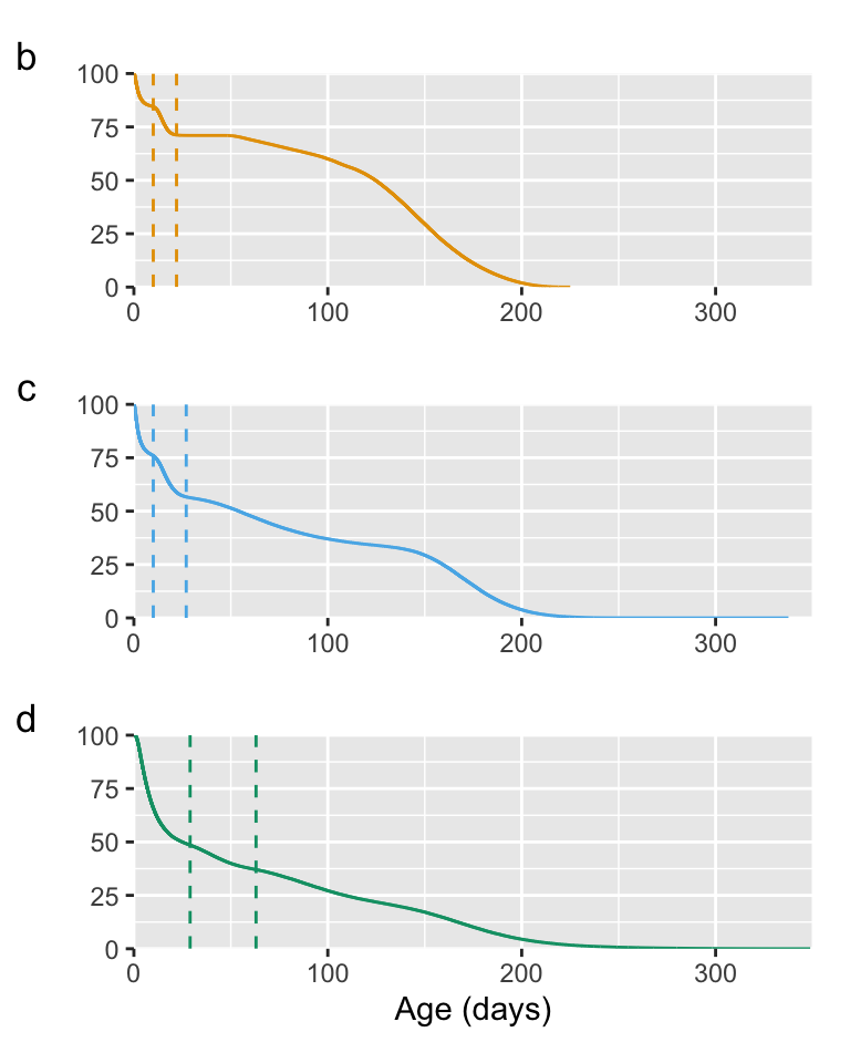
# plotting each species separately as well
p1<-ggplot(data=plot_datatest[plot_datatest$strata=="vannamei",],
                         aes(x=time, y=estimate*100, color=strata)) +
  geom_line(color="#E69F00") +
  labs(y="") +
  scale_x_continuous(limits=c(0,350),
                     expand = c(0, 0)) +
  scale_y_continuous(expand = c(0, 0)) +
  theme(legend.position="none", plot.margin=unit(c(b=0.5,t=0.5,r=0.5, l=0), "lines"),
        axis.title.x=element_blank()) +
  #scale_color_manual(values=c("#E69F00","#56B4E9","#009E73")) +
  geom_vline(xintercept=10, linetype="dashed", colour="#E69F00") + # cell NX in the Guesstimate model
  geom_vline(xintercept=22, linetype="dashed", colour="#E69F00") # cell DA in the Guesstimate model

p2<-ggplot(data=plot_datatest[plot_datatest$strata=="monodon",],
                         aes(x=time, y=estimate*100)) +
  geom_line(color="#56B4E9")+
  labs(y="")+
  scale_x_continuous(limits=c(0,350),
                     expand = c(0, 0)) +
  scale_y_continuous(expand = c(0, 0)) +
  theme(legend.position="none",
        plot.margin=unit(c(b=0.5,t=0.5,r=0.5, l=0), "lines"),
        axis.title.x=element_blank()) +
  geom_vline(xintercept=10, linetype="dashed", colour="#56B4E9") + # cell LQ in the Guesstimate model
  geom_vline(xintercept=27, linetype="dashed", colour="#56B4E9") # cell HJ in the Guesstimate model

p3<-ggplot(data=plot_datatest[plot_datatest$strata=="Macrobrachium",],
                         aes(x=time, y=estimate*100)) +
  geom_line(color="#009E73")+
  labs(x="Age (days)", y="") +
  scale_x_continuous(limits=c(0,350),
                     expand = c(0, 0)) +
  scale_y_continuous(expand = c(0, 0)) +
  theme(legend.position="none",
        plot.margin=unit(c(b=0.5,t=0.5,r=0.5, l=0), "lines"),
        axis.title.y=element_blank()) +
  geom_vline(xintercept=29, linetype="dashed", colour="#009E73") + # cell OD in the Guesstimate model
  geom_vline(xintercept=63, linetype="dashed", colour="#009E73") # cell TK in the Guesstimate model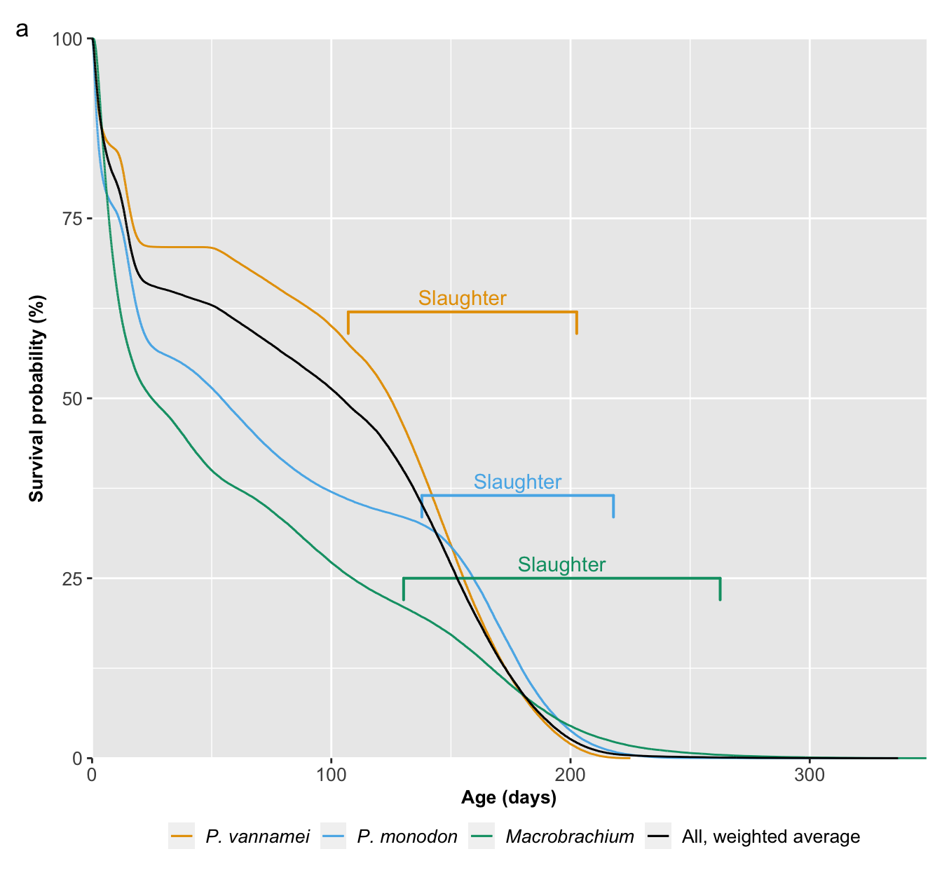

We also extract the average probability of making it to slaughter age for each species:

mean(vannamei_stage_probabilities[,4])

[1] 0.5902775

mean(monodon_stage_probabilities[,4])

[1] 0.3225594

mean(macro_stage_probabilities[,4])

[1] 0.1914582

1.4 Comparing to slaughter statistics

We next compare the slaughter figures to the number that died on farms (including pre-slaughter mortality) in the same year.

slaughter<-read.csv("../data/guesstimate/slaughtered_samples.csv")

vannamei_slaught<-slaughter$vannamei %>% 
  kde1d() %>%
  rkde1d(100000,.)
give.summary(slaughter$vannamei, vannamei_slaught) %>%
  add_header_above(c("P. vannamei" = 3))
monodon_slaught<-slaughter$monodon %>% 
  kde1d() %>%
  rkde1d(100000,.)
give.summary(slaughter$monodon, monodon_slaught) %>%
  add_header_above(c("P. monodon" = 3))
macro_slaught<-slaughter$macrobrchium %>% 
  kde1d() %>%
  rkde1d(100000,.)
give.summary(slaughter$macrobrchium, macro_slaught) %>%
  add_header_above(c("Macrobrachium" = 3))
allspecies_slaught<-cbind(vannamei_slaught, monodon_slaught, macro_slaught) # combining the 100,000 samples for each species into a data frame

slaught_prop_allspecies<-as.data.frame(allspecies_slaught) %>% 
  rowwise() %>%
  mutate(van_prop=vannamei_slaught/sum(vannamei_slaught, monodon_slaught, macro_slaught), # calculating each sample as a proportion of the total shrimp, row-wise
         mon_prop=monodon_slaught/sum(vannamei_slaught, monodon_slaught, macro_slaught),
         macro_prop=macro_slaught/sum(vannamei_slaught, monodon_slaught, macro_slaught))

P. vannamei
	original	new
5%	220957800000	222476066766
50%	342228500000	343470146341
95%	529217650000	532874614636
mean	354766329600	356150888840
sd	96851040159	96858142911
min	144325000000	104518134351
max	952712000000	987182924790

P. monodon
	original	new
5%	11860315356	11923173880
50%	20858815142	20984152771
95%	36622412461	36434870776
mean	22092898841	22176970451
sd	7815695540	7784774999
min	5996479921	4618419389
max	71459992373	73715081829

Macrobrachium
	original	new
5%	20277647900	20563786382
50%	31033290274	31051657941
95%	46842577016	46844762225
mean	31986343208	32058892477
sd	8291128218	8209105772
min	10376290701	10599353581
max	86753502536	87744803041

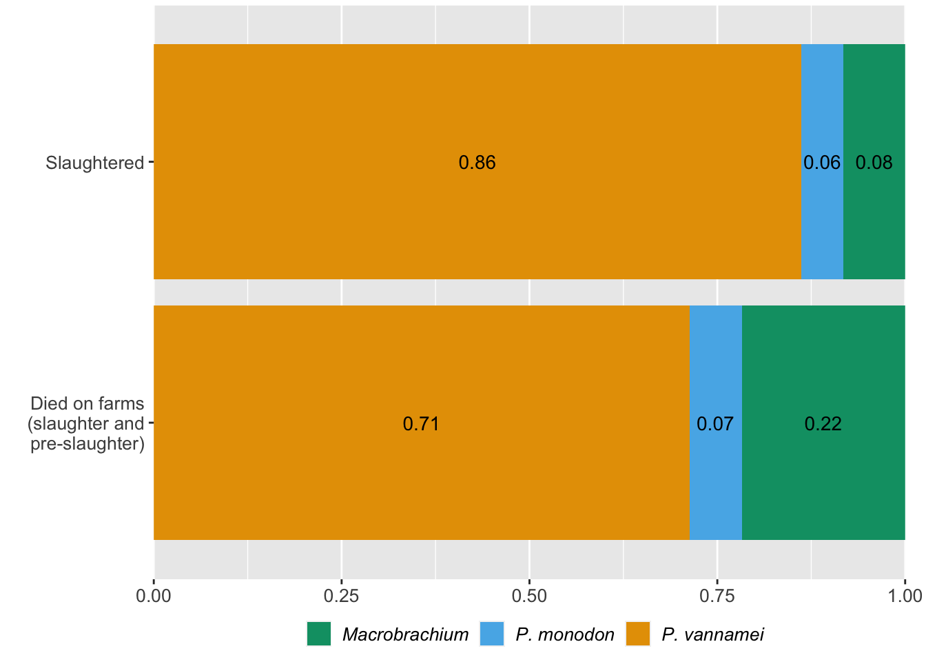
Now we can compare the proportion of farmed shrimp from each species that are slaughtered annually and that die on farms annually.

# make all the data of interest into a data frame
comp_slaught_dof<-data.frame(Species=rep(c("vannamei", "monodon", "macrobrachium"), 2), 
                             Type=c(
                               rep("Slaughtered", 3),
                               rep("Die on farms (including pre-slaughter mortality)", 3)),
                             Proportion=c(
                               mean(slaught_prop_allspecies$van_prop),
                               mean(slaught_prop_allspecies$mon_prop),
                               mean(slaught_prop_allspecies$macro_prop), 
                               mean(prop_allspecies_dof$van_prop),
                               mean(prop_allspecies_dof$mon_prop),
                               mean(prop_allspecies_dof$macro_prop)),
                             Lower=c(
                               quantile(slaught_prop_allspecies$van_prop, probs=0.025),
                               quantile(slaught_prop_allspecies$mon_prop, probs=0.025),
                               quantile(slaught_prop_allspecies$macro_prop, probs=0.025),
                               quantile(prop_allspecies_dof$van_prop, probs=0.025),
                               quantile(prop_allspecies_dof$mon_prop, probs=0.025),
                               quantile(prop_allspecies_dof$macro_prop, probs=0.025)),
                             Upper=c(
                               quantile(slaught_prop_allspecies$van_prop, probs=0.975),
                               quantile(slaught_prop_allspecies$mon_prop, probs=0.975),
                               quantile(slaught_prop_allspecies$macro_prop, probs=0.975),
                               quantile(prop_allspecies_dof$van_prop, probs=0.975),
                               quantile(prop_allspecies_dof$mon_prop, probs=0.975),
                               quantile(prop_allspecies_dof$macro_prop, probs=0.975)))

# plot the results as individual bars
ggplot(comp_slaught_dof, aes(y=Type, x=Proportion, fill=Species)) +
  geom_bar(stat="identity", position="dodge") +
  geom_errorbar(aes(xmin=Lower, xmax=Upper), position=position_dodge(width=.9), width=.7) +
  scale_fill_manual(values=c("#009E73","#56B4E9",  "#E69F00"), 
                    labels=c(
                      expression(italic("Macrobrachium")),
                      expression(italic("P. monodon")),
                      expression(italic("P. vannamei")))) +
  scale_x_continuous(expand=c(0,0), limits=c(0,1)) +
  scale_y_discrete(labels=c("Died on farms\n(including\npre-slaughter\nmortality)", "Slaughtered")) +
  theme(legend.text = element_text(hjust=0)) +
  ylab("") +
  xlab("Proportion") 
# plot as stacked bars
ggplot(comp_slaught_dof, aes(y=Type, x=Proportion, group=Species, fill=Species)) +
  geom_bar(stat="identity", position="stack") +
  geom_text(aes(label=round(Proportion, 2)),stat="identity",position=position_stack(vjust=.5), color="black", size=3.7) +
  scale_fill_manual(values=c("#009E73","#56B4E9",  "#E69F00"), 
                    labels=c(expression(italic("Macrobrachium")), expression(italic("P. monodon")), expression(italic("P. vannamei")))) +
  scale_x_continuous(expand=c(0,0), limits=c(0,1)) +
  scale_y_discrete(labels=c("Died on farms\n(slaughter and\npre-slaughter)", "Slaughtered")) +
  theme(legend.position="bottom",
        legend.title=element_blank(),
        legend.key.size = unit(5, "mm"),
        legend.text=element_text(size=10, hjust=0),
        legend.spacing.x = unit(2, "mm"),
        axis.text=element_text(size=10),
        axis.title.y=element_text(size=10, face="bold"),
        axis.title.x=element_blank(),
        legend.box.spacing = unit(1, "mm"),
        plot.margin = unit(c(1,4,1,1), "mm")) +
  ylab("") +
  xlab("Mean proportion")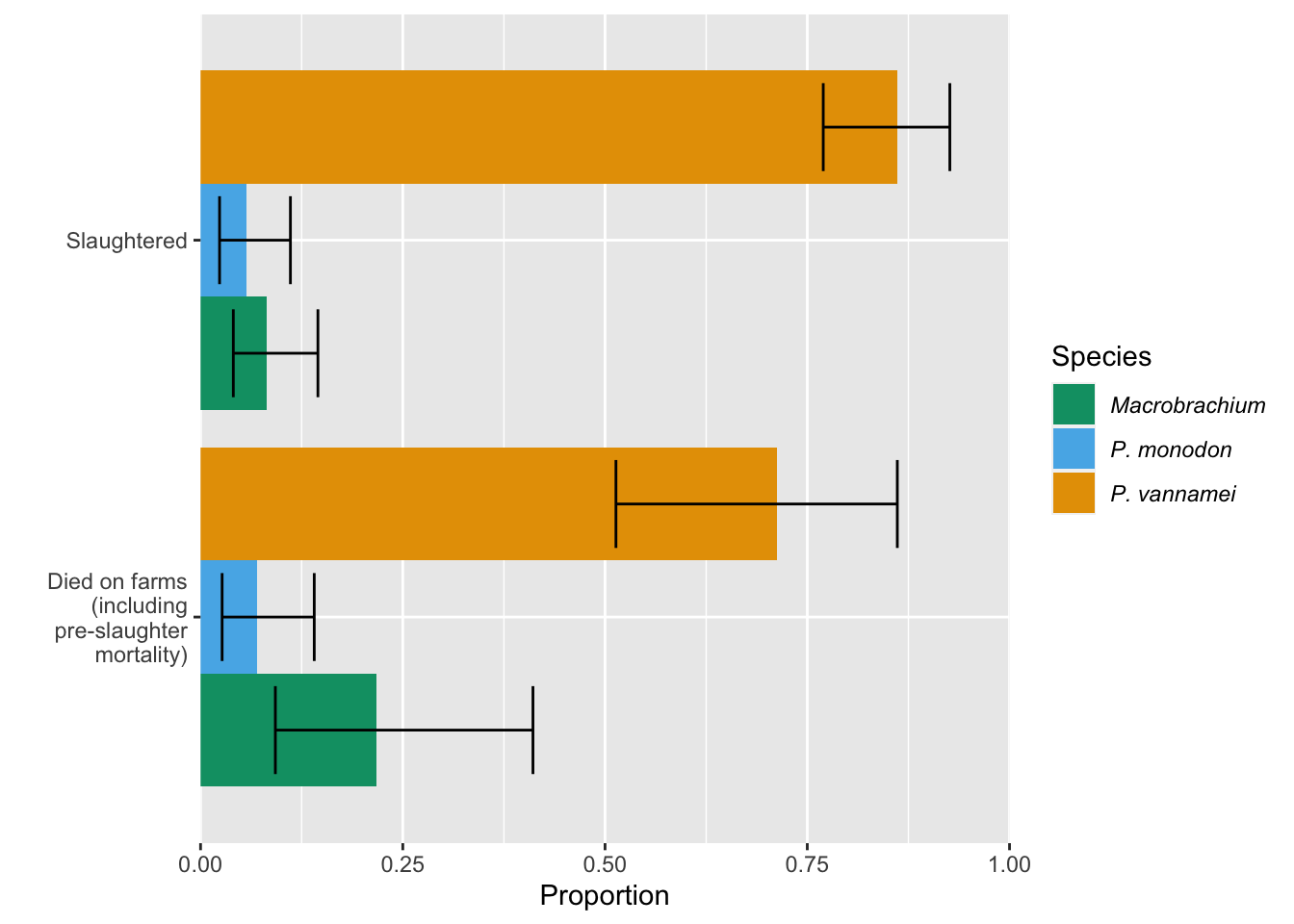

1.5 Stage specific rates and numbers of individuals

Finally, we extract the mean and 95% credible intervals for mortality rate at each life stage (including cumulative mortality rate) and number of individuals who die on farms at each stage (and in total).

# calculate individual deaths for each life stage of each species
van_total_larval_deaths<-mean(vannamei_dof)*mean(vannamei_stage_prob$larval)
van_left_after_larval<-mean(vannamei_dof)-van_total_larval_deaths
van_total_postlarval_deaths<-van_left_after_larval*mean(vannamei_stage_prob$postlarval)
van_left_after_postlarval<-van_left_after_larval-van_total_postlarval_deaths
van_total_juvenile_deaths<-van_left_after_postlarval*mean(vannamei_stage_prob$juvenile.adult)
van_left_after_juvenile<-van_left_after_postlarval-van_total_juvenile_deaths
van_total_psm<-mean(vannamei_dof)*(1-mean(vannamei_stage_probabilities[,4]))

mon_total_larval_deaths<-mean(monodon_dof)*mean(monodon_stage_prob$larval)
mon_left_after_larval<-mean(monodon_dof)-mon_total_larval_deaths
mon_total_postlarval_deaths<-mon_left_after_larval*mean(monodon_stage_prob$postlarval)
mon_left_after_postlarval<-mon_left_after_larval-mon_total_postlarval_deaths
mon_total_juvenile_deaths<-mon_left_after_postlarval*mean(monodon_stage_prob$juvenile.adult)
mon_left_after_juvenile<-mon_left_after_postlarval-mon_total_juvenile_deaths
mon_total_psm<-mean(monodon_dof)*(1-mean(monodon_stage_probabilities[,4]))

macro_total_larval_deaths<-mean(macro_dof)*mean(macro_stage_prob$larval)
macro_left_after_larval<-mean(macro_dof)-macro_total_larval_deaths
macro_total_postlarval_deaths<-macro_left_after_larval*mean(macro_stage_prob$postlarval)
macro_left_after_postlarval<-macro_left_after_larval-macro_total_postlarval_deaths
macro_total_juvenile_deaths<-macro_left_after_postlarval*mean(macro_stage_prob$juvenile.adult)
macro_left_after_juvenile<-macro_left_after_postlarval-macro_total_juvenile_deaths
macro_total_psm<-mean(macro_dof)*(1-mean(macro_stage_probabilities[,4]))

# make a data frame of the required data
mort_indivs<-data.frame(
  species=c(rep("P. vannamei", 4), rep("P. monodon", 4), rep("Macrobrachium", 4)),
  stage=rep(c("Larval", "Postlarval", "Juvenile-subadult", "Cumulative"), 3),
  mortality_mean=c(
    mean(vannamei_stage_prob$larval),
    mean(vannamei_stage_prob$postlarval),
    mean(vannamei_stage_prob$juvenile.adult),
    (1-mean(vannamei_stage_probabilities[,4])),
    mean(monodon_stage_prob$larval),
    mean(monodon_stage_prob$postlarval),
    mean(monodon_stage_prob$juvenile.adult),
    (1-mean(monodon_stage_probabilities[,4])),
    mean(macro_stage_prob$larval),
    mean(macro_stage_prob$postlarval),
    mean(macro_stage_prob$juvenile.adult),
    (1-mean(macro_stage_probabilities[,4]))
  ),
  mortality_lower=c(
    quantile(vannamei_stage_prob$larval, probs=0.025),
    quantile(vannamei_stage_prob$postlarval, probs=0.025),
    quantile(vannamei_stage_prob$juvenile.adult, probs=0.025),
    (1-quantile(vannamei_stage_probabilities[,4], probs=0.975)),
    quantile(monodon_stage_prob$larval, probs=0.025),
    quantile(monodon_stage_prob$postlarval, probs=0.025),
    quantile(monodon_stage_prob$juvenile.adult, probs=0.025),
    (1-quantile(monodon_stage_probabilities[,4], probs=0.975)),
    quantile(macro_stage_prob$larval, probs=0.025),
    quantile(macro_stage_prob$postlarval, probs=0.025),
    quantile(macro_stage_prob$juvenile.adult, probs=0.025),
    (1-quantile(macro_stage_probabilities[,4], probs=0.975))
  ),
  mortality_upper=c(
    quantile(vannamei_stage_prob$larval, probs=0.975),
    quantile(vannamei_stage_prob$postlarval, probs=0.975),
    quantile(vannamei_stage_prob$juvenile.adult, probs=0.975),
    (1-quantile(vannamei_stage_probabilities[,4], probs=0.025)),
    quantile(monodon_stage_prob$larval, probs=0.975),
    quantile(monodon_stage_prob$postlarval, probs=0.975),
    quantile(monodon_stage_prob$juvenile.adult, probs=0.975),
    (1-quantile(monodon_stage_probabilities[,4], probs=0.025)),
    quantile(macro_stage_prob$larval, probs=0.975),
    quantile(macro_stage_prob$postlarval, probs=0.975),
    quantile(macro_stage_prob$juvenile.adult, probs=0.975),
    (1-quantile(macro_stage_probabilities[,4], probs=0.025))
  ),
  individuals_mean=c(
    van_total_larval_deaths,
    van_total_postlarval_deaths,
    van_total_juvenile_deaths,
    van_total_psm,
    mon_total_larval_deaths,
    mon_total_postlarval_deaths,
    mon_total_juvenile_deaths,
    mon_total_psm,
    macro_total_larval_deaths,
    macro_total_postlarval_deaths,
    macro_total_juvenile_deaths,
    macro_total_psm
    )
)

# add brackets to show the 95% credible intervals
mort_indivs$Mortality<-paste0(
  round(mort_indivs$mortality_mean, 2), " [", 
  round(mort_indivs$mortality_lower, 2), "; ", 
  round(mort_indivs$mortality_upper, 2), "]")

mort_indivis_pivot<-mort_indivs %>%
  pivot_wider(id_cols = species, names_from = stage, values_from = c(Mortality, individuals_mean))

transpose_mort_indivis_pivot<-t(mort_indivis_pivot)

# print the results
kbl(transpose_mort_indivis_pivot) %>%
  kable_styling(full_width=F, position="center", font_size=9, bootstrap_options = c("condensed"))

species	P. vannamei	P. monodon	Macrobrachium
Mortality_Larval	0.16 [0.09; 0.25]	0.25 [0.19; 0.31]	0.54 [0.38; 0.74]
Mortality_Postlarval	0.16 [0.09; 0.24]	0.25 [0.19; 0.31]	0.18 [0.09; 0.34]
Mortality_Juvenile-subadult	0.17 [0.04; 0.48]	0.43 [0.03; 0.97]	0.49 [0.38; 0.62]
Mortality_Cumulative	0.41 [0.27; 0.65]	0.68 [0.44; 0.98]	0.81 [0.71; 0.9]
individuals_mean_Larval	97014532629	13814892071	96844873542
individuals_mean_Postlarval	81691380200	10489285669	15388806842
individuals_mean_Juvenile-subadult	76747517895	13643028391	33677996607
individuals_mean_Cumulative	255431609229	37946354695	145914976464

1.6 Data and method limitations

The data underpinning the survival curves does not account for broodstock (shrimp used as breeders). The figures also likely miss some small-scale or illegal farms and may not include “failed crops” with mass mortality due to, for example, diseases. The number of individuals is also sensitive to the inputted individual weight of shrimp, but data is scarce for this metric and slaughter weight likely changes over time and between locations. For a complete description of the limitations of the Monte-Carlo Guesstimate model which underpins our survival curves, see the appendix in Waldhorn and Autric (2023).