3 Engagement

firstup <- function(x) {
  substr(x, 1, 1) <- toupper(substr(x, 1, 1))
  x
}

#moved to build side
# eas_20 <- eas_20 %>% sjlabelled::var_labels(engagement_num = "Engagement",
#                age_approx = "Age",
#                tenure = "Time in EA",
#                age_first_inv = "Age first-involved in EA")

scatter_theme <- theme_minimal()

Note: This chapter presents (most) of the material from our EAS 2020: Engagement EA forum post, along with the code and dynamic graphs. The chapter goes into more technical depth than the EA forum post, and presents some additional work and results. (However, some of the material from the forum post is not here, particular where it was created directly in Google Sheets; this is noted and linked below.

This work also connects to the work in a previous post/chapter on “Do introducers predict and/or drive engagement?”

See also our 2019 post on the same topic

3.1 Introduction

We describe people’s self-reported levels of engaged in EA, what activities related to effective altruism they have completed and their group membership. We also describe differences in these modes of engagement across groups (gender, race, age, time in EA etc.) and present a series of models looking at factors associated with higher engagement.

This hosted ‘bookdown’ content covers this in more detail, with folded code and some dynamic depictions.

3.1.1 Why do we care about ‘engagement?’

2019 introduction:

In recent years there has been significant interest in the levels of engagement of EAs and in particular, the most engaged members of the community. The focus and resources devoted to those considered “contributors” or “core”(1, 2) (add links) are likely very different to those considered part of the EA “network.” CEA has noted that the level of involvement with EA of typical applicants to EA Globals has risen so much that the typical person who didn’t get accepted to attend has changed from someone who was barely involved with EA to someone who is probably pretty knowledgeable about EA and has been involved for at least a few years.

These points remain relevant. We present a descriptive picture of “who is more engaged” because this offers greater understanding of “what the EA movement looks like.” Those who are more engaged are likely to have a greater impact, and thus may be of greater interest for some considerationss.

In addition to description, we are also interested in more ambitious predictive and even (at least suggestively) causal modeling of engagement for several reasons, also mentioned in previous posts. These serve three categories of goals Outreach, Planning, and Policy.

1. Outreach: Knowing “who is likely to become engaged” may inform decisionmaking surrounding ‘how much resources to devote to recruiting and supporting EAs,’ and ‘at which age to recruit EAs’ (see further analysis of the latter question below. This motivates a predictive approach: trying to forecast (lifetime) engagement based on factors (e.g., age, career background, source of ‘first heard of EA’) that can be measured, and are fixed at a point in time before the engagement and involvement journey. (Unfold further discussion…)

“EA lifetime value?”….

In other words, this can help movement and group leaders (and active EAs) make better decisions about how many resources to put into recruiting and retaining people from different areas and in different ways. One might make an analogy to “customer lifetime value” in marketing – companies will offer more costly promotions to those customers they think will be more valuable over the long term. This is not necessary the way we want to view this; it is just one perspective.

Prediction and extrapolation; modeling concerns…

If we know ‘which sorts of people were more likely to become engaged’ in the past, this may predict ‘which sorts… that we might recruit now, are likely to become engaged in the future.’ Of course, we should be careful about making these extrapolations, as the nature of background processes may change over time, as well as the links between an observed and observed factors.

For example, ‘jazzy people’ in the years 2014-2016 may have tended to also have being a highly prosocially motivated, because the jazz movement was volunteer-based during this period. Thus, being jazzy in 2015 may have been highly predictive of EA engagement in 2020. But if the jazz movement started to pay people to join in 2020, then being jazzy in 2020 may poorly predict EA engagement in 2025.

Differential attrition issue…

Another factor that limits this: If we use only the 2020 survey, these estimates may be driven by differential attrition from EA, and from filling out the survey, as noted elsewhere.

Suppose we find that people who are inherently jazzy (for simplicity, suppose this is an immutable characteristic), who we see in the 2020 survey, tend to be much more highly engaged. This could be because being jazzy is closely linked to engagement, or to another unobserved factor that predicts engagement. In such a case, we may expect this to be a good predictor of future engagement, and this would argue for us trying to heavily recruit jazzy people. However, another possibility is that jazzy people tend to only continue in the movement and fill out the surveys when they are heavily engaged, while non-jazzy people fill out the surveys equally regardless of their engagement level. We can only disentangle this by looking at earlier data and considering the differential rates of attrition.

We have some evidence for differential rates of attrition, e.g., by ‘introducer’ – see Attrition from EA/EA survey by introducer in the “How EAs get Involved in EA” post.

We are still considering how how to feasibly deal with this as we have fairly low rates of reseponses where people share their emails and thus limited connectivity across years. E.g., on average, an individual in any EA survey can be tracked over only 1.3 surveys.

From fold: E.g., on average, an individual in any EA survey can be tracked over only 1.3 surveys 1.31290397944085 surveys)

Taking into account both engagement and attrition, over a medium run, this will also inform decisions surrounding “whether and how much to encourage growth,” and how much to “focus on helping those already in the movement take further actions.” A key measure informing this decision is the “conversion rate” between new recruits to EA (who tend to be less engaged. and later heavily engaged EAs.

Caveat: Diversity and other concerns…

‘Likelihood of becoming engaged’ may not be the only, or even the principle concern; recruiting diverse EAs from a variety of contexts is likely to be a goal in itself, and may also unlock new networks, opportunities, and approaches.

2. Planning and anticipating movement growth: How is EA (and engagement) likely to grow over time, and in what ways? (Unfold further discussion…)

We may want to know how large the movement is likely to grow over time, and what level of engagement we can predict in the future. This could inform choices we make about infrastructure as well as which approaches to focus on. For example (hypothetically), if it is unlikely that we will ever become a large and engaged movement, this may make direct political action less feasible and less worth planning, and we might be less concerned about the dilution of core ideas. Knowing what the composition of the movement is likely to look like in the future (e.g., age, demographics and geography) may also help identify more fruitful possibilities. The EA Survey may help us learn the ways the different participants tend to become more or less engaged over time, as well as whether they leave the movement entirely. This may allow better forecasting and planning.

3. Policy/what works: Knowing “what might lead to people becoming more engaged” will help us choose which approaches to take in bringing people into the movement, encouraging their participation, and promoting different activities and messages. However, this causal inference is a harder target.

4. Policy/what works: Knowing “what might lead to people becoming more engaged” will help us choose ‘policies,’ i.e., understand which approaches to take in bringing people into the movement, encouraging their participation, and promoting different activities and messages. However, this causal inference is a harder target (discussed in fold).

To the extent that we do observe the ‘policies’ an individual EA faced (or things related to these, like the self-reported influences). These will tend to be related to other observable and unobservable characteristics (such as country, age, year-joined, individual’s educational choices), which in turn may have direct and indirect effects and relate to other important on observable determinants of engagement.

As we do not have clear policy experiments or ‘natural experiments’ (see the literature on causal inference), we can, at best, look for patterns that suggest causal links. Because of this limitation, we will do this only sparingly in the current post/chapter.

3.2 Measures of Engagement

3.2.1 Engagement measures and validation

As stated in 2019:

It is important to state at the outset that being involved in the community by posting on the Forum, attending lots of events, or working at EA related organizations is not necessarily the same as dedication to EA or having the most impact.

Here we examine how engaged in different activities are the 2,513 EAs who responded to the 2019 EA Survey. Naturally, what measure we should use to determine the most engaged EAs in the survey is controversial. Any proxy we select will also necessarily be imperfect as there will almost certainly be exceptions to the rule. In this post we examine potential proxies, which may each capture distinct modes of EA involvement; group membership, activities, and self-reported engagement.

For the current post (for the 2020 survey) we focus on self-reported engagement.

We give a simple table of self-reported engagement below:

eas_20 %>%
  tabyl(engagement) %>% adorn_pct_formatting(digits = 2) %>% .kable() %>% .kable_styling()

engagement	n	percent	valid_percent
No engagement	44	2.14%	2.40%
Mild engagement	352	17.12%	19.19%
Moderate engagement	549	26.70%	29.93%
Considerable engagement	544	26.46%	29.66%
High engagement	345	16.78%	18.81%
NA	222	10.80%

#eas_20 %>% tabyl(engagement_num, referrer_cat)

In a separate document linked HERE we present our work assessing whether the self-report engagement is meaningfully related to the behavior that are intuitively associated with engagement. The analysis strongly supports this association.

3.3 Descriptives of engagement (see forum post [LINK])

The content in this section was mainly created in created in Google Sheets. Thus we link the forum post here, rather than presenting it again.

eas_20_m <- eas_20 %>% select(
  engagement,
starts_with("action")) %>%
reshape2::melt(id.vars="engagement")  %>%
mutate(counter=1) %>%
group_by(engagement, variable) %>%
  summarise(share =  mean(as.numeric(value), na.rm=TRUE))

eas_20_m %>%
ggplot(aes(x = engagement, y = share, fill = variable)) +
  geom_bar(stat = "identity") +
  coord_flip()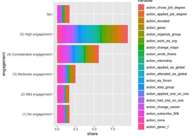

3.4 Descriptives: Engagement by Demographics, Socio-Economic factors, Attitudes/Behaviors, and Paths (and vice-versa)

3.4.1 Self-reported engagement: key comparisons

We consider differences in key characteristics by level of engagement. We first present a numerical table summarizing a key set of socio-demographics, priorities, and behaviors; we present these both overall and for each level of self-reported engagement.

(
  demo_tab_engagement <- eas_20 %>%
       mutate(engage_cats_1 = as.factor(engage_cats_1),
                  engage_cats_1= fct_drop(engage_cats_1)
              ) %>%
    select(all_of(key_outcomes), engage_cats_1, -engagement_num) %>%
    tbl_summary(
      by = engage_cats_1,
       type = c(all_continuous(), mn_priority_lt_rating, don_share_inc_19_imp) ~ "continuous2",
      statistic = list(all_continuous() ~ c("{median}",
                                            "{p10}-{p90}",
                                            "{mean} ({sd})"),
                       all_dichotomous() ~ "{p}%"),
      label = label_list[1:11],
      missing = c("no"),
          digits = list(mn_priority_lt_rating ~1)
    ) %>%
    modify_spanning_header(c("stat_1", "stat_2", "stat_3", "stat_4") ~ "**Self-reported engagement**") %>%
 modify_footnote(
    update = all_stat_cols() ~ "*See notes in text.") %>%
   bold_labels() %>% add_n() %>% add_overall()
)

Characteristic	N	Overall, N = 1,8341	Self-reported engagement
			1-2, N = 3962	3, N = 5492	4, N = 5442	5, N = 3452
Age	1,604
Median		27	30	28	26	28
10%-90%		21-41	21-55	21-41	20-34	22-37
Mean (SD)		30 (10)	35 (14)	30 (10)	27 (7)	29 (7)
Male	1,574	71%	62%	71%	73%	73%
Student	1,635	37%	29%	35%	46%	32%
White (ethnicity)	1,600	83%	84%	82%	83%	84%
USA-based	1,606	39%	36%	40%	39%	39%
Income in $1000	1,409
Median		33	44	37	22	33
10%-90%		1-130	0-125	1-143	1-120	3-122
Mean (SD)		61 (137)	56 (75)	66 (133)	55 (124)	65 (192)
Academic current career	1,620	18%	16%	17%	20%	19%
Mean prioritization LT (1-5)	1,584
Median		3.4	3.0	3.2	3.4	3.5
10%-90%		2.3-4.0	2.0-4.0	2.2-4.0	2.5-4.0	2.6-4.2
Mean (SD)		3.3 (0.7)	3.0 (0.8)	3.2 (0.7)	3.4 (0.6)	3.4 (0.6)
LT cause(s) highest	1,614	51%	38%	47%	58%	58%
Animal welfare highest	1,549	19%	14%	15%	26%	17%
Donation as share of income, with imputation	1,422
Median		0.02	0.01	0.02	0.03	0.04
10%-90%		0.00-0.14	0.00-0.10	0.00-0.12	0.00-0.22	0.00-0.20
Mean (SD)		0.12 (1.78)	0.05 (0.13)	0.05 (0.12)	0.10 (0.38)	0.32 (3.95)
1 c("Median", "10%-90%", "Mean (SD)"); % 2 *See notes in text.

Notes on the above table…*

** This table removes respondents who didn’t report their engagement. ‘Mean prioritization LT’ averages the priority assigned to X-risk, AI risks, Biosecurity, Nuclear, and broad-LT-ism’; ‘LT cause(s) highest’ indicates that one of these causes was among those the individual ranked most-highly.

In the above table Gender, (White) ethnicity, student status and academic career don’t seem to have a strong relationship to engagement. The least-engaged seem somewhat older, more female, less likely to be students, and less USA-based. The less-engaged also appear to be less long-termist. The most-engaged seem to donate a larger share of their income. Other patterns are less clear: median income seems to decline in engagement somewhat, while mean income is fairly constant.

3.4.2 Summary charts

Descriptive measures also help us locate ‘where the engaged people are,’ and help us compare which groupings are more engaged. Below, we present ‘relative frequency stacked bar charts’ showing the ‘raw’ (uncontrolled) relationships between key characteristics and the levels of self-reported engagement. All bars are grouped from ‘highest to lowest share with 4-5 engagement,’ except for age, which is grouped by youngest to oldest. The bars depict 95% confidence intervals for the ‘shares of each subgroup with 4-5 engagement,’ as well as the narrower 1-standard-error bars.

mutate_eng <- function(df) {
{df} %>%
  filter(!is.na(engagement)) %>%
        mutate(engagement= fct_recode(engagement,
                              "(1) None" = "(1) No engagement",
                             "(2) Mild" = "(2) Mild engagement" ,
                             "(3) Moderate" = "(3) Moderate engagement",
                             "(4) Considerable" = "(4) Considerable engagement",
                             "(5) High" = "(5) High engagement",
                             ))
}


engage_stack_layers <- list(
  geom_bar(aes(fill=engagement), position="fill"),
    theme(axis.title.x = element_blank(),
          axis.text.x = element_blank(),
          axis.ticks.x = element_blank(),
          axis.ticks.y = element_blank(),
          axis.title.y = element_blank()
    ),
  stat_summary(aes(y = engage_high_n),
           fun.data = mean_cl_normal,  na.rm = TRUE,
           geom = "errorbar", colour = "pink", width = 0.2),
stat_summary(aes(y = engage_high_n),
           fun.data = mean_cl_normal,  na.rm = TRUE,
           geom = "errorbar",  colour = "purple", width = 0.2,
           fun.args = list(mult = 1)),
     coord_flip()
      )

engage_by_age <- eas_20 %>%
  mutate_eng %>%
    ggplot() +
 aes(x = fct_rev(age_approx_ranges) ) +
  engage_stack_layers +
    labs(title = "Engagement x 'Age'", x="Age", y="share", caption = "95% CI bars for 'share 4-5 engaged'  in pink, 1 SE in purple")

engage_by_gender <- eas_20 %>% filter(!is.na(engagement)) %>%
    ggplot() +
 aes(x = reorder(gender_cat, engage_high_n) ) +
  engage_stack_layers +
    labs(title = "... x Gender", x="Gender", y="share")

  engage_by_student <- eas_20 %>% filter(!is.na(engagement)) %>%
    ggplot() + aes(x = reorder(student_cat,  engage_high_n) ) + engage_stack_layers +
    labs(title = "... x Student", x="Student", y="share")

  engage_by_race <- eas_20 %>% filter(!is.na(engagement)) %>%
    ggplot() + aes(x = reorder(race_cat,  engage_high_n) ) + engage_stack_layers +
    labs(title = "... x Ethnicity", x="Ethnicity", y="share")


  engage_by_where_live_cat <- eas_20 %>% filter(!is.na(engagement)) %>%
    ggplot() + aes(x = reorder(where_live_cat,  engage_high_n) ) + engage_stack_layers +
    labs(title = "... x Location", x="Where live", y="share")


  engage_by_city_cat <- eas_20 %>% filter(!is.na(engagement)) %>%
    ggplot() + aes(x = reorder(city_cat,  engage_high_n) ) + engage_stack_layers +
    labs(title = "...  x (Named) big city", x="Big", y="share")


(
  engage_by_cat_stack <- ggarrange(engage_by_age, engage_by_gender, engage_by_student, engage_by_race, engage_by_where_live_cat, engage_by_city_cat,
                    ncol = 2, nrow = 3,
                    heights = c(1, 1),
                    align = "v",
                      common.legend = TRUE, legend = "bottom")
)

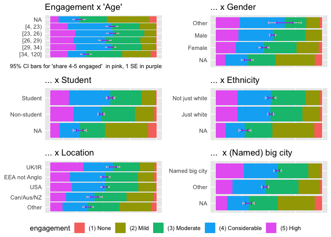
Examining the proportion of respondents who self-identified as levels 1-3 vs 4-5 in terms of engagement, we observe that:

• Those >34 years of age reported being less engaged

• Male respondents reported being more engaged

• Students reported being more engaged

• Those living in one of the 22 big cities named in the survey ^[These were cities known to have relatively high EA populations: Amsterdam, Auckland, Berlin, Boston / Cambridge (USA), Cambridge (UK) , Canberra, Chicago, London Los Angeles Melbourne, New York City, Oslo, Oxford, Philadelphia, Seattle, SF Bay Area, Stockholm, Sydney, Toronto, Vienna, Washington DC, Zürich] reported being more engaged

• In terms of country of residence groupings, UK + Ireland were the most engaged, and Canada + Australia + New Zealand the least engaged.

3.4.3 When people get involved in EA/ Time in EA / Age / Age When First Involved in EA

This subsection, given in the Forum post, is mainly subsumed by the Engagement: age, tenure, period and cohort effects subsection below.

3.4.4 Gender and self-reported engagement, … and group membership - see forum post [LINK]

3.4.5 Race and and group membership; Race and activities - see forum post

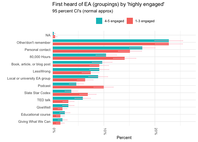
3.4.6 Where people first heard of EA

We analyzed differences in engagement between respondents who reported first hearing about EA from different sources in this earlier post and section. For a quick reference, we give a breakdown of engagement by groups of ’where first heard of EA’below (this is a simpler version of a chart presented in “How EAs get involved in EA”).

dodge_thing <- list(
  geom_bar(position=position_dodge2(), stat='identity'),
  scale_fill_hue(labels = c("1-3 engaged", "4-5 engaged" ) ),
  theme_minimal(),
  guides(fill=guide_legend(title=NULL)),
  theme(legend.position = "top"),
  guides(fill = guide_legend(title=NULL, reverse = TRUE)),
  theme(axis.text.x = element_text(angle = -90, vjust = 0, hjust=0)),
  scale_y_continuous(labels=percent, expand = expansion(mult = c(0,.1))),
  coord_flip()
  )

p_load(binom)
p_load(standardize)

fh_45_data_l <- eas_20 %>%
  select(d_engage_4_5, first_hear_ea_lump) %>%
    filter(!is.na(d_engage_4_5)) %>%
    group_by(d_engage_4_5, first_hear_ea_lump) %>%
    mutate(fheg_n = n()) %>%
      group_by(d_engage_4_5) %>%
        mutate(eng_n = n()) %>%
         unique() %>%
     mutate(fheg_share = fheg_n/eng_n) %>%
      mutate(eg_share_se = sqrt((fheg_share*(1-fheg_share))/eng_n)) %>%
    ungroup()

ci_s <- binom.confint(x=fh_45_data_l$fheg_share*fh_45_data_l$eng_n, n=fh_45_data_l$eng_n, methods="wilson")


fh_45_data_l <- cbind(fh_45_data_l, ci_s[,5:6])

(
  fh_e45_plotl <-  fh_45_data_l %>%
  ggplot() +
  aes(x = reorder(first_hear_ea_lump,fheg_share), fill=d_engage_4_5,  y = fheg_share) +
    dodge_thing +
     geom_errorbar(aes(ymin=fheg_share-1.96*eg_share_se, ymax=fheg_share+1.96*eg_share_se), width=.2,  colour = "pink", position=position_dodge(.9)) +
  labs(title = "First heard of EA (groupings) by 'highly engaged'", subtitle = "95 percent CI's (normal approx)", y = "Percent", x = "")
)

3.5 Modeling engagement*

* This section slightly overlaps some of the material in our “How EAs get involved” post.

3.5.1 Descriptive modeling

As mentioned in the introduction, we care “what is associated with engagement holding other things constant?” Although much of our analysis is merely meant to be descriptive, in general we try to leave out ‘confounders’ (especially things that are themselves proxies for engagement). However. we recognize that ‘being in the sample’ (considering attrition) may be a sort of confounder in itself.

3.5.2 Predictive and causal modeling

As noted in the introduction [LINK], predictive and/or causal models inform Outreach, Planning, and Policy.

We seek to build models that predict…

1. Accurately:

• predicting outside the data the model was trained on (see the problem of “Overfitting”),

• and predicting throughout the range of the years of data, including the most recent data (Allowing for trends and trend-differences across years may make the model better at predicting well in the future.)

2. …Based on variables we can and do observe at the time we make relevant policy choices. Thus:

• considering the limits of the EAS scope, and

• without using ‘ex-post’ and ‘outcome’ variables such as ‘participation in EA Forum’ (aka ‘leaks’ and ‘colliders’).

3. …For EA individuals, not just for the subset of individuals who remain in EA/in the EA survey. Thus:

• We need to take attrition (from EA and from the survey) seriously, and potentially make it part of our model.
  

3.5.2.1 Ideal (future) modeling approach

Ideally we would, and will… (unfold)

I. Create a measure \(G\) (or set of measures) of ‘engagement’ (and or value-added) that captures the outcomes we think we are looking for. Previous ‘clustering’ work (by Kim) may inform this.

For the present, we will use “self-reported engagment (or dichotomising this into 1-3 vs 4-5).” As noted above, this measure seems to be ‘validated’ by the cluster analysis.

2. Goals and relationships (theoretical structural model)

In a perfect world, we would like to estimate a function

• for the (real or counterfactual) ‘level of engagement’
• of person \(i\) in year \(t\),
• with permanent characteristics \(X_i\) and time-varying characteristics \(X_{it}\) (these are vectors),
• who became involved in EA in year \(t_0\),
• who was ‘exposed to a vector \(S_t\) of EA stimuli in each year since joining,’ summarized as \(S \equiv S_t \forall t \geq t_0\).

We can write this ‘true structural model’ as

\[G_{it} = f(t, X_i, X_{it}, S, t_0, t) + \epsilon_{it}\],

where \(\epsilon_{it}\) is an irreducible true random term.

In principle, knowing the above ‘true model’….

… would allow us to address a range of causal questions about possible ‘interventions,’ e.g.,

how engaged would the average German Female who joins EA in 2021 be in 2025 if they were (A) exposed to a heavy diet of LessWrong and three 80K podcasts per month … versus (B) if they were not exposed to Less Wrong but (induced?) to taking the GWWC pledge and becoming vegan. Thus “what is the (causal) effect of (B) relative to (A)?”

or similar ‘retrospective’ questions:

… who joined EA in 2014 have been in 2020 if they had been exposed to some set of stimuli (C) versus (D)? (Or if they had joined in 2015 instead, etc.)

More reasonably, we will never be able to observe all of the important characteristics of the individual, nor her exposures, never know the ‘true functional form’ of the model, nor be able to perfectly distinguish causal relationships from chance. (But we will do our best!)

We aim for a more ‘predictive model’ first, while considering issues of causality.

For example, considering the previous questions, we may aim to predict…

What will be the average level of engagement for a typical individual whom we see, in year 0, in observable group \(A\), after \(\tau=5\) years of being in EA’? How does the same measure differ from that of an individual whom we see in group \(B\)?

I.e., \[E\big(G_{t_0+5}|A\big) - E\big(G_{t_0+5}|B\big)\]

Consider “group,” to embody any number of characteristics we observe in the EAS, such as ‘place first heard of EA,’ or ‘country of origin.’ Here we are not asking the causal ‘counterfactual’ question ‘for the same individual how would this differ depending on whether they were in (or had the characteristics of) group A versus B, all else equal.’ All else is not equal: we realize that for any groupings A and B, people in these groups will have very different observable and unobservable characteristics (\(X_i, X_{it}\)) from one another, and also will be exposed to a different set of stimuli \(S\).*

* They may also have joined EA in different calendar years (\(t_0\)), but we will explicitly try to keep this constant in our work.

Instead, we will focus on making decent predictions to guide our policy choices.

One might we mainly care most about making these predictions for people entering in future years, so as to better direct our resources (see above discussion of the ‘three goals’). Knowing that ‘EAs who joined through GWWC in 2014 are more active (in 2021) than those who joined through LW in 2017’ only informs our choices to the extent that these differences are stable, and likely to persist into future years.

Choices of variables/features

Prediction and outreach strategies: There are a range of categories on which we might want to make policy-relevant predictions about engagement. We may care specifically about the extent to which other things (demographics, initial alignment, etc) predict later engagement.

In assessing the impact of a factor such as ‘introducer,’ a causal model might reasonably ‘control’ for other observable features, such as age and gender.*

* However, causal interpretation will still require strong assumptions, and ‘controls’ can sometimes introduce additional bias to causal estimates.

On the other hand, a predictive model may not want to ‘control’ in the same way. Suppose we were specifically considering the potential of each (e.g., ‘first-heard’) ‘channel’ in recruiting EEAs. Here, e.g., we may want to know whether LessWrong can be expected to outperform 80K allowing that part of this difference may be driven by age or gender differences. Here we might not want to “difference out” the component of the LW effect that comes from these.**

** However, we might bring this decomposition back in a mixed-modeling context.

We focus on a few of these below

Predictors (and/or causal factors) of interest for outreach questions

• ‘Place first heard of EA’

• Demographics, geography, other identifiable characteristics

For forecasting growth (and as ‘controls’ in interpreting the predictive features)

We have not (yet) built a full ‘growth model.’ However, the features below may be informative and suggestive.

• Year entered EA (‘Cohort’): Particularly important in considering the aggregated retrospective data

• Time in EA (Tenure; hard to distinguish from cohort)

• Period (‘when’ we are seeing the level of engagement)

However, it is difficult to separate period, cohort and tenure/age effects in general as well as in our specific case.

In general, \(Period = Cohort + Tenure\); we cannot identify the ‘effect’ of all three of these independently, without any further restrictions.

For 2020 retrospective data, \(Period=2020\) and \(Cohort = 2020 - Tenure\). Unless we are willing to make further assumptions (e.g., a linear impact of Tenure), we will necessarily pick up cohort and tenure effects together.*

* I discuss ‘Traditional APC and APCC models’ further in my notes here … see “Age-period-cohort effects”… which I hope to expand.

More broadly, the growth of ‘engaged EA’ will depend on recruitment rates, attrition, on how people’s engagement changes with with tenure, and whether there are cohort (and secular period) trends towards less/more engagement.

Choosing features and modeling target variables

(Code below: I define a series of feature sets for modeling, and maybe define the contrast codings and labelings)

#targets:
bin_out <- "d_engage_4_5"
num_out <- "engagement_norm"
cat_out <- "engagement"

geog <- c("where_live_cat", "city_cat")

key_demog <- c("age_approx_d2sd", "gender_cat", "student_cat", "race_cat", geog)
big_demog <- c("age_approx_d2sd", "female_cat",  "student_cat", "race_cat", "usa_cat", "city_cat")

#removed 'current career' as that seems closely tied to engagement ergo a potential confounder
#removed  "d_straight" because there is so much nonresponse there, and I think responding to that signals a high degree of engagement

#Add: elite university, country regions

#predictors
key_predictors <- c(key_demog)
controls <- c("years_involved_d2sd") #note this assumes those 2009 or earlier started in 2009
robust_controls <- c("year_involved_groups", "age_approx_ranges")
possible_endog <- c("income_d2sd", "uni_higher_rank_d2sd", "d_pt_employment", "d_not_employed", "d_retired")
other_predictors <- c("first_hear_ea_lump")

eas_20 %>% sm("d_live|d_not_em|straight|big_city|uni_higher_rank_d2sd") %>% vtable::sumtable()

(#tab:feature_sets)Summary Statistics

Variable	N	Mean	Std. Dev.	Min	Pctl. 25	Pctl. 75	Max
d_not_employed	1636	0.049	0.216	0	0	0	1
d_live_usa	1607	0.386	0.487	0	0	1	1
uni_higher_rank_d2sd	1073	0	0.5	-1.897	-0.178	0.343	0.383

#“no big city” — named ‘other’ as their city.
#d_straight — that’s low because so many people didn’t answer this question
#career_other: that’s not student nor full time employed

#contrasts(normtimeBP02$Nasality) = contr.treatment(4)

(Code below: Imputing and normalizing)

#note: rescaling work moved to eas_stata_to_r_clean.R

eas_20_s <- eas_20 %>%
  dplyr::select(all_of(c(num_out, cat_out, bin_out, key_predictors, "usa_cat", "female_cat", controls, robust_controls,  possible_endog, other_predictors)))

eas_s_nomissing <- eas_20_s %>%
  select(all_of(c(cat_out, key_predictors, controls))) %>%
filter_all(all_vars(str_detect(as.character(.), pattern = "NA", negate = TRUE))) %>%
  gdata::drop.levels() %>%
  mutate(
where_live_cat = relevel(as.factor(where_live_cat), ref="USA"),
        city_cat = relevel(as.factor(city_cat), ref="Other"),
    student_cat = relevel(as.factor(student_cat), ref="Non-student"),
    gender_cat = relevel(as.factor(gender_cat), ref="Male"),
      race_cat = relevel(race_cat, ref="Just white")
  )

#missing_to_zero: moved to R-stuff functions.R thing

#Recode missing as 0 for all dummies, as a 'NA category' for categoricals
#also for normalized variables; i.e., set missings to the mean
eas_20_s <- eas_20_s %>%
    mutate(across(matches("d_|not_just_white"), missing_to_zero))

eas_20_s_imp <- eas_20_s %>%
      mutate(across(matches("d2sd"), missing_to_zero))

eas_20_s_imp %>% vtable::sumtable()

(#tab:impute_norm_features)Summary Statistics

Variable	N	Mean	Std. Dev.	Min	Pctl. 25	Pctl. 75	Max
engagement_norm	1834	0	1	-2.269	-0.404	0.529	1.461
engagement	1834
… (1) No engagement	44	2.4%
… (2) Mild engagement	352	19.2%
… (3) Moderate engagement	549	29.9%
… (4) Considerable engagement	544	29.7%
… (5) High engagement	345	18.8%
d_engage_4_5	2056	0.432	0.496	0	0	1	1
age_approx_d2sd	2056	0	0.442	-1.31	-0.242	0.063	3.673
gender_cat	2056
… Male	1112	54.1%
… Female	423	20.6%
… NA	481	23.4%
… Other	40	1.9%
student_cat	2056
… Non-student	1035	50.3%
… NA	420	20.4%
… Student	601	29.2%
race_cat	2056
… Just white	1223	59.5%
… NA	454	22.1%
… Not just white	379	18.4%
where_live_cat	2056
… USA	621	30.2%
… Can/Aus/NZ	178	8.7%
… EEA not Anglo	456	22.2%
… Other	572	27.8%
… UK/IR	229	11.1%
city_cat	2056
… Other	839	40.8%
… NA	507	24.7%
… Named big city	710	34.5%
usa_cat	2056
… USA	621	30.2%
… Not USA	1435	69.8%
female_cat	2056
… Not female	1152	56%
… Female	423	20.6%
… NA	481	23.4%
years_involved_d2sd	2056	0	0.463	-0.585	-0.398	0.165	1.477
year_involved_groups	1761
… 2014 or before	287	16.3%
… 2015-16	385	21.9%
… 2017-18	525	29.8%
… 2019-20	564	32%
age_approx_ranges	1605
… [4, 23)	313	19.5%
… [23, 26)	290	18.1%
… [26, 29)	278	17.3%
… [29, 34)	387	24.1%
… [34, 120]	337	21%
income_d2sd	2056	0	0.414	-0.221	-0.156	0	10.71
uni_higher_rank_d2sd	2056	0	0.361	-1.897	0	0.227	0.383
d_pt_employment	2056	0.034	0.181	0	0	0	1
d_not_employed	2056	0.039	0.193	0	0	0	1
d_retired	2056	0.018	0.131	0	0	0	1
first_hear_ea_lump	1839
… Other/don’t remember	420	22.8%
… 80,000 Hours	228	12.4%
… Book, article, or blog post	173	9.4%
… Educational course	35	1.9%
… GiveWell	45	2.4%
… Giving What We Can	32	1.7%
… LessWrong	151	8.2%
… Local or university EA group	141	7.7%
… Personal contact	300	16.3%
… Podcast	135	7.3%
… Slate Star Codex	97	5.3%
… TED talk	82	4.5%

Ordered logit models of self-reported engagement level

We consider the association between a range of features and the respondent’s level of engagement. These (arguably) should still not be interpreted as causal relationships.

Below, we construct an ordered logit model, reporting the odds ratios. As noted in our ‘community information’ post, these can be loosely interpreted as the “relative probability of stating a 1 unit higher level of satisfaction,” relative to the base group.

Interpreting these estimates…

E.g., if the coefficient for ‘jazzy’ is 1.5, this means that, controlling for everything else in the model, comparing any two levels of engagement (2 versus 1, 5 versus 4, etc) jazzy people are approximately 50% more likely to be in the higher group. Note that the ordered logit model imposes a particular functional form: a variable must have proportional relative ‘effect’ on the probability of being in a higher versus a lower category, with this proportional ‘effect’ being the same between any comparison of adjacent categories. However, a strong justification can be made that this is ‘more realistic’ than a linear model, which interprets the 1-5 engagement self report as if it were a meaningful cardinal outcome.

ol_mdl <- function(df, rhs) {
  polr(
    m_f(cat_out, {{rhs}}), data = df, Hess = TRUE
    ) %>%
    broom::tidy(conf.int = TRUE, exponentiate = TRUE) %>%
  filter(coef.type=="coefficient")  %>%
    dplyr::arrange(-str_detect(term, 'd2sd')) %>%
      mutate(
        term = str_replace_all(term, c("where_live_cat" = "Where live: ",
                                       "d2sd" = " (2 sd norm.)",
                                       "gender_cat" = "Gender: ",
                                       "female_catFemale" = "Female (vs. non-female)",
                                       "student_catNA" = "Student: NA",
                                       "student_cat" = "",
                                       "city_catNA" = "City: NA",
                                       "city_cat" = "",
                                       "usa_catNA" = "Where live: NA",
                                       "usa_cat" = "",
                                       "race_catNA" = "Race: NA",
                                       "race_cat" = "",
                                       "age_approx_" ="Age",
                                       "uni_higher_rank_" = "Univ. rank (+)",
                                       "years_involved" = "Years Involved EA",
                                       "d_retired" = "Retired",
                                       "d_" = "",
                                       "first_hear_ea_lump" = "1st heard EA: ",
                                       "pt_employment" = "Part-time Employed",
                                       "not_employed" = "Not Employed",
                                       "income_" ="Income",
                                       "Giving What We Can" = "GWWC",
                                       "Slate Star Codex" = "SSC"
                                       )
                              )
      )
}


rename_eng_mod_list <-  c("where_live_cat" = "Where live: ",
                                       "d2sd" = " (2 sd norm.)",
                                       "gender_cat" = "Gender: ",
                                       "female_catFemale" = "Female (vs. non-female)",
                                       "student_catNA" = "Student: NA",
                                       "student_cat" = "",
                                       "city_catNA" = "City: NA",
                                       "city_cat" = "",
                                       "usa_catNA" = "Where live: NA",
                                       "usa_cat" = "",
                                       "race_catNA" = "Race: NA",
                                       "race_cat" = "",
                                       "age_approx_" ="Age",
                                       "uni_higher_rank_" = "Univ. rank (+)",
                                       "years_involved" = "Years Involved EA",
                                       "d_retired" = "Retired",
                                       "d_" = "",
                                       "first_hear_ea_lump" = "1st heard EA: ",
                                       "pt_employment" = "Part-time Employed",
                                       "not_employed" = "Not Employed",
                                       "income_" ="Income",
                                       "Giving What We Can" = "GWWC",
                                       "Slate Star Codex" = "SSC"
                                       )

require("parallel")

clean_model_p <- function(polr_results) {
  parallel::mclapply(polr_results,  function(x) {
    broom::tidy(x, conf.int = TRUE, exponentiate = TRUE) %>%
      filter(coef.type=="coefficient")
  })
}

ol_engage_naive_m <- eas_20_s_imp %>%  polr( m_f(cat_out, c(key_predictors)), data = ., Hess = TRUE )

ol_engage_naive <- eas_20_s_imp %>% ol_mdl(c(key_predictors))

ol_engage_noimp_m <- eas_20_s %>%  polr( m_f(cat_out, c(key_predictors, controls)), data = ., Hess = TRUE )
ol_engage_noimp <- eas_20_s %>%  ol_mdl(c(key_predictors, controls))


ol_engage_nomissing_m <- eas_s_nomissing %>%
  polr(m_f(cat_out, c(key_predictors, controls)), data = ., Hess = TRUE )

ol_engage_imp_m <- eas_20_s_imp %>% polr(m_f(cat_out, c(key_predictors, controls)), data = ., Hess = TRUE)
ol_engage_imp <- eas_20_s_imp %>% ol_mdl(c(key_predictors, controls))


##Do: with more robust controls : year_involved_groups, age_approx_ranges
ol_engage_imp_m_r <- eas_20_s_imp %>% polr(m_f(cat_out, c(key_predictors, controls, robust_controls)), data = ., Hess = TRUE)
ol_engage_imp_r <- eas_20_s_imp %>% ol_mdl(c(key_predictors, controls, robust_controls))

ol_engage_imp_big_m <- eas_20_s_imp %>% polr(m_f(cat_out, c(big_demog,  controls)), data = ., Hess = TRUE)
ol_engage_imp_big <- eas_20_s_imp %>%
  ol_mdl(c(big_demog,  controls))

ol_engage_possible_endog_m <- eas_20_s_imp %>%  polr(m_f(cat_out, c(key_predictors, controls, possible_endog)), data = ., Hess = TRUE)
ol_engage_possible_endog <- eas_20_s_imp %>%
    ol_mdl(c(key_predictors, controls, possible_endog))

fh_imp_n <- eas_20_s_imp %>% smn("first_hear")

ol_engage_fh_imp_m <- eas_20_s_imp %>% polr(m_f(cat_out, c(key_predictors, controls, fh_imp_n)), data = ., Hess = TRUE)
ol_engage_fh_imp <- eas_20_s_imp %>%
    ol_mdl(c(key_predictors, controls, fh_imp_n))

#pseudo-r-sq

ol_engage_imp_m_nag_pr2 <-  DescTools::PseudoR2(ol_engage_imp_m, which = "Nagelkerke")

ol_engage_noimp_m_nag_pr2 <-  DescTools::PseudoR2(ol_engage_noimp_m, which = "Nagelkerke")


# Models to tidy tibbles for use in plots

ol_engage_tidymod <- clean_model_p(
  list(
        "(0) Naive" = ol_engage_naive_m,
        "(1) Baseline" = ol_engage_imp_m,
        "(1a) Baseline - no imputation" = ol_engage_noimp_m,
        "(1b) Larger groupings" = ol_engage_imp_big_m,
        "(4) Possibly endogenous" = ol_engage_possible_endog_m,
        "(5) First-heard" = ol_engage_fh_imp_m,
        "Robust controls" = ol_engage_imp_m_r
    )
)

ol_na_terms <- ol_engage_possible_endog_m$term[grepl("NA", ol_engage_possible_endog_m$term)]

ol_key_pred_n_ctn <- grep("d2sd", names(coef(ol_engage_imp_m)), value = TRUE)
ol_key_pred_n_cat <- grep("first_hear_ea_lump|Intercept|NA|d2sd", names(coef(ol_engage_imp_m)), value = TRUE, invert=TRUE)

ol_na_pred <- grep("NA|Intercept", names(coef(ol_engage_imp_m)), value = TRUE)
names(ol_na_pred) <- gsub("_cat", ": ", ol_na_pred) %>%
  gsub("student", "Employment status", . ) %>%
  firstup(.)

ol_key_pred_n <- c(ol_key_pred_n_ctn, ol_key_pred_n_cat)
names(ol_key_pred_n) <- gsub("where_live_cat", "Live: ", ol_key_pred_n ) %>%
  gsub("age_approx_d2sd", "Age (2 sd norm.)",. ) %>%
    gsub("uni_higher_rank_d2sd", "Uni. rank (+)", .) %>%
 gsub("d2sd", "(2 sd norm.)", .) %>%
  gsub("student_catStudent", "Student", .) %>%
  gsub("cat", "- ", .)  %>%
  #gsub("canzaus", "Aus///Can///NZ", .) %>%
  gsub("city_-","", .) %>%
  firstup(.) %>%
  gsub("D_", "", .) %>%
  gsub("Race_- ", "", .) %>%
  gsub("_", " ", .) %>%
  firstup(.) %>%
  gsub("Pt", "PT", .)

fh_n <- grep("first_hear_ea_lump", names(coef(ol_engage_fh_imp_m)), value = TRUE)
names(fh_n) <- gsub("first_hear_ea_lump", "First-heard: ", fh_n)   %>%
    gsub("X80", "80", .)  %>%
    gsub("Giving What We Can", "GWWC", .) %>%
    gsub("Slate Star Codex", "SSC", .) %>%
    gsub("Book, article, or blog post", "Book/article/blog", .) %>%
    gsub("Local or university EA group", "Local/Univ. EA group", .)


names_pos_endog =c("Income (2sd norm)" = "income_d2sd",
                   "Univ. (+) rank, (2sd norm)" = "uni_higher_rank_d2sd" ,
                    "Retired" =  "d_retired",
                    "PT Employment" = "d_pt_employment" ,
                    "Not Employed" = "d_not_employed"
                   )

names_big <-  c("Binary: Female (vs. non-female)" = "female_catFemale",
                      "Binary: Not USA-based)" = "usa_catNot USA"
                        )

(
  ol_engage_tbl_m <- huxreg(
        "(1) Baseline" = ol_engage_imp_m,
        "(2) Possibly endogenous" = ol_engage_possible_endog_m,
        "(3) First-heard" = ol_engage_fh_imp_m,
      tidy_args = list(conf.int = TRUE, prob = 0.95, exponentiate =TRUE),
      coefs = c(ol_key_pred_n,  names_pos_endog,
              fh_n
              ),
     number_format = 2,
    statistics = c("N. obs." = "nobs"),
    error_pos = "right", ci_level = .95, error_format = "({conf.low}, {conf.high})") %>%
        huxreg_opts %>%
    set_col_width(c(1, rep(c(0.4, 0.4), times=5))) %>%
        set_caption("Ordered logistic models <br> Odds-ratios; 95% CI's in parentheses; NA ratios hidden") %>%
  set_caption_pos("top")  %>%
    head(-1) #get rid of missing p-value thing
  )

(#tab:ol_eng_rename_hux) Ordered logistic models
Odds-ratios; 95% CI's in parentheses; NA ratios hidden

	(1) Baseline		(2) Possibly endogenous		(3) First-heard
Age (2 sd norm.)	0.37	(0.30, 0.46)	0.37	(0.29, 0.47)	0.37	(0.29, 0.46)
Years involved (2 sd norm.)	4.46	(3.66, 5.45)	4.44	(3.64, 5.43)	4.52	(3.67, 5.57)
Gender - Female	0.80	(0.65, 0.98)	0.79	(0.64, 0.97)	0.72	(0.58, 0.89)
Gender - Other	1.04	(0.58, 1.86)	1.00	(0.56, 1.79)	0.98	(0.54, 1.75)
Student	1.30	(1.05, 1.61)	1.34	(1.07, 1.67)	1.25	(1.01, 1.55)
Not just white	0.99	(0.79, 1.23)	0.98	(0.78, 1.23)	1.00	(0.80, 1.25)
Live: Can/Aus/NZ	0.83	(0.61, 1.13)	0.82	(0.60, 1.11)	0.83	(0.61, 1.14)
Live: EEA not Anglo	1.26	(0.99, 1.60)	1.26	(0.99, 1.60)	1.20	(0.94, 1.53)
Live: Other	1.60	(1.13, 2.27)	1.61	(1.14, 2.29)	1.51	(1.06, 2.15)
Live: UK/IR	1.44	(1.09, 1.92)	1.41	(1.06, 1.87)	1.41	(1.05, 1.89)
Named big city	1.56	(1.28, 1.92)	1.56	(1.27, 1.91)	1.53	(1.24, 1.87)
Income (2sd norm)			0.95	(0.77, 1.17)
Univ. (+) rank, (2sd norm)			1.17	(0.94, 1.47)
Retired			1.03	(0.51, 2.06)
PT Employment			1.04	(0.67, 1.61)
Not Employed			1.54	(1.00, 2.38)
First-heard: 80,000 Hours					0.76	(0.56, 1.02)
First-heard: Book/article/blog					1.10	(0.79, 1.53)
First-heard: Educational course					1.84	(0.94, 3.65)
First-heard: GiveWell					1.23	(0.68, 2.21)
First-heard: GWWC					0.61	(0.30, 1.28)
First-heard: LessWrong					0.79	(0.56, 1.12)
First-heard: Local/Univ. EA group					1.16	(0.82, 1.64)
First-heard: Personal contact					1.18	(0.90, 1.56)
First-heard: Podcast					0.89	(0.62, 1.27)
First-heard: SSC					0.48	(0.32, 0.73)
First-heard: TED talk					1.22	(0.79, 1.88)
N. obs.	1834.00		1834.00		1828.00

In the Ordered Logit models summarized in the above table, continuous variables (income, age, university rank) are de-meaned and divided by two standard-deviations.*

* This is for comparability to dummy-coded categorical variables, see Gelman, 2007. Where these are missing they are coded as zero, the mean of the transformed variable.

Base groups are set as the most numerous group in each category. Thus, all dummy coefficients represent adjustments from the ‘overall base group’: an individual who is male, works full-time, ‘just White’ ethnicity, USA-based, not based in a (survey-named) big city, and ‘first heard of EA’ response is ‘other or don’t remember.’

The above models include dummy variable ‘controls’ for nonresponses to each of the given categorical variables. These coefficients are hidden in the above table, but shown further below.

We next present a forest plot of the coefficients from the baseline model, considering only ex-ante factors (with imputation):*

* It is important to note that these are in multivariable models. Thus, while the odds-ratio shifter for ‘Where live: Other’ is among the most positive, this does not imply that the most-engaged EA’s are necessarily in these other countries.

We next present a forest plot of the coefficients from the baseline model, considering only ex-ante factors (with imputation).

library(ggstatsplot)

(
ol_engage_imp_tree <- ol_engage_imp %>%
    filter(!grepl("NA|Ageranges|year_involvegroups",term)) %>%
  ggstatsplot::ggcoefstats(statistic=t,
              sort="ascending",
              stats.labels = "TRUE",
              title = "Engagement: ex-ante associated factors",
              subtitle = "Ordered logit model, 95% CI's; NA ratios hidden",
              vline=FALSE) +
  ggplot2::labs(
        x= NULL,
        y = "Characteristics (normalized)"
      ) +
      geom_vline(xintercept=1, colour="grey") +
    geom_text(aes(x=1, label="Odds=1", y=10), colour="brown", angle=90, vjust = -.9) +
      scale_x_continuous(trans='log2', limits=c(0.25, 8))
) %>%
  ggplotly()

Next, we present a similar forest plot of the model that includes some characteristics that may not be strictly ex-ante (model 2 in the first table):

(
  ol_engage_possible_endog_tree <-  ol_engage_possible_endog %>%
        filter(!grepl("NA$",term)) %>%
  ggcoefstats(statistic=t,
              sort="ascending",
              stats.labels = "TRUE",
              title = "Engagement: associated factors ",
              subtitle = "Ordered logit model, 95% CI's; Model '(4) Possibly endogenous'; NA ratios hidden",
              vline=FALSE) +
  ggplot2::labs(
        x= NULL,
        y = "Characteristics (normalized)"
      ) +
      geom_vline(xintercept=1, colour="grey") +
    geom_text(aes(x=1, label="Odds=1", y=12), colour="brown", angle=90, vjust = -.9) +
      scale_x_continuous(trans='log2', limits=c(0.25, 7.5))
) %>%
  ggplotly()

Nonresponse: The table below presents the coefficients from a selection of the above models, on the ‘lack of a response to’ (i.e., skipping) certain questions.

Finally the table below presents the coefficients (from a selection of the above models) on the ‘lack of a response to’ (i.e., skipping) certain questions.

(
  ol_engage_tbl_na <- huxreg(
        "(1) Baseline " = ol_engage_imp_m,
        "(2) Baseline - no imputation" = ol_engage_noimp_m,
        "(4) Possibly endogenous" = ol_engage_possible_endog_m,
      "(5) First-heard" = ol_engage_fh_imp_m,
           tidy_args = list(conf.int = TRUE, prob = 0.95, exponentiate = TRUE),
            coefs = c(ol_na_pred),
     number_format = 2,
    statistics = c("N. obs." = "nobs"),
    error_pos = "right", ci_level = .95, error_format = "({conf.low},  {conf.high})") %>%
        huxreg_opts %>%
    set_caption("Engagement: Ordered logistic models <br> NA Odds-ratios; 95% CI's in parentheses") %>%
  set_caption_pos("top")
  #%>% head(-1) #get rid of missing p-value thing
  )

Table 3.1: Engagement: Ordered logistic models
NA Odds-ratios; 95% CI's in parentheses

	(1) Baseline		(2) Baseline - no imputation		(4) Possibly endogenous		(5) First-heard
Gender: NA	0.56	(0.33, 0.97)	0.58	(0.31, 1.08)	0.54	(0.32, 0.94)	0.57	(0.33, 0.99)
Employment status: NA	0.90	(0.47, 1.75)	3.27	(0.56, 21.35)	0.90	(0.47, 1.76)	0.83	(0.43, 1.60)
Race: NA	0.54	(0.27, 1.08)	0.52	(0.20, 1.31)	0.55	(0.27, 1.11)	0.54	(0.27, 1.09)
City: NA	0.93	(0.61, 1.41)	0.77	(0.49, 1.20)	0.94	(0.62, 1.44)	1.00	(0.66, 1.52)
N. obs.	1834.00		1604.00		1834.00		1828.00
*** p < 0.001; ** p < 0.01; * p < 0.05.

This nonresponse seems to largely be associated with less engagement, particularly for the race/ethnicity question. However, non-response to the ‘location’ question seems to be an exception, perhaps because the base group, USA-residence, tends to be lower-engagement.

3.5.3 Interpretation, robustness, further exploration

Comparison across ordered logit models, adjusting variable choices and transformations

We next present a series of similar (ordered logistic) models to delve more deeply into what is driving the above, and test robustness.

(
  ol_engage_tbl_m_compare <- huxreg(
        "(0) Naive" = ol_engage_naive_m,
        "(1) Baseline " = ol_engage_imp_m,
        "(1a) Baseline - no imputation" = ol_engage_noimp_m,
        "(1b) Larger groupings" = ol_engage_imp_big_m,
      tidy_args = list(conf.int = TRUE, prob = 0.95, exponentiate =TRUE),
        coefs = c(ol_key_pred_n,
                names_big
                  ),
     number_format = 2,
    statistics = c("N. obs." = "nobs"),
    error_pos = "right", ci_level = .95, error_format = "({conf.low},  {conf.high})") %>%
        huxreg_opts %>%
    set_col_width(c(1, rep(c(0.4, 0.4), times=4))) %>%
    set_caption("Comparisons: Ordered logistic models <br> Odds-ratios; 95% CI's in parentheses; NA ratios hidden") %>%
  set_caption_pos("top")  %>%
    head(-1) #get rid of missing p-value thing
  )

(#tab:ol_eng_compare) Comparisons: Ordered logistic models
Odds-ratios; 95% CI's in parentheses; NA ratios hidden

	(0) Naive		(1) Baseline		(1a) Baseline - no imputation		(1b) Larger groupings
Age (2 sd norm.)	0.42	(0.34, 0.52)	0.37	(0.30, 0.46)	0.36	(0.28, 0.44)	0.36	(0.29, 0.45)
Years involved (2 sd norm.)			4.46	(3.66, 5.45)	4.51	(3.66, 5.58)	4.48	(3.68, 5.47)
Gender - Female	0.72	(0.58, 0.88)	0.80	(0.65, 0.98)	0.80	(0.65, 0.99)
Gender - Other	1.23	(0.70, 2.16)	1.04	(0.58, 1.86)	1.05	(0.59, 1.89)
Student	0.89	(0.72, 1.09)	1.30	(1.05, 1.61)	1.27	(1.02, 1.58)	1.28	(1.04, 1.59)
Not just white	0.93	(0.75, 1.16)	0.99	(0.79, 1.23)	1.02	(0.81, 1.28)	1.03	(0.83, 1.27)
Live: Can/Aus/NZ	0.71	(0.52, 0.97)	0.83	(0.61, 1.13)	0.86	(0.62, 1.17)
Live: EEA not Anglo	1.12	(0.88, 1.41)	1.26	(0.99, 1.60)	1.28	(1.00, 1.63)
Live: Other	1.28	(0.90, 1.80)	1.60	(1.13, 2.27)	1.56	(1.08, 2.25)
Live: UK/IR	1.46	(1.10, 1.92)	1.44	(1.09, 1.92)	1.44	(1.08, 1.91)
Named big city	1.77	(1.45, 2.16)	1.56	(1.28, 1.92)	1.60	(1.30, 1.97)	1.51	(1.24, 1.83)
Binary: Female (vs. non-female)							0.79	(0.64, 0.97)
Binary: Not USA-based)							1.24	(1.03, 1.50)
N. obs.	1834.00		1834.00		1604.00		1834.00

Column (0) presents a ‘naive’ model that does not control for time-in-EA. this model may be helpful as a description of the engagement levels of those currently in EA. However, it is confounded with differences that are driven by the changing nature of recruitment into the movement, as is not likely to be predictive (nor causal). Nonetheless, we mostly do not see strong differences from our baseline model, presented (again) in column (1). This does seeem to impact the odds-ratio for ‘Students.’ The naive model suggests students are less engaged, while the baseline model suggests they are engaged at about the same rate as others, given their (typically shorter) tenure in EA.*

* The control for ‘years in EA’ also had a more substantial effect on the coefficients of the different ‘first-heard’ coefficients in column (3) of the previous table.

Column (1a) repeats the base model, but dropping (rather than imputing) participants that did not respond to the age or ‘years involved’ questions (note the smaller number of observations). These results are very close to the base model.**

** We also ran a comparable model that dropped all cases with missing values for any of the variables in this mode. Again, the results (available by request) are largely similar.

Column 1b adjusts the baseline model to use larger groupings. The results here suggest that those based in the USA are less engaged, controlling for other factors. (Other results are similar to previously-reported columns).

These models are only able to “explain” a moderate share of the variation in engagement (but note we did not choose the models parameters to maximize this. The pseudo-r-sq for above models (Nagelkerke method) is 0.17 and 0.15 for the “(1) Baseline” and “(2) Baseline - no imputation,” respectively. The comparable statistic for most of the other models is close to that of model (1).

Pseudo-r-sq for above models (Nagelkerke method):

ol_engage_imp_m_nag_pr2

## Nagelkerke 
##   0.241454

ol_engage_noimp_m_nag_pr2

## Nagelkerke 
##  0.2180222

For the “(1) Baseline” and “(2) Baseline - no imputation,” respectively. The comparable statistic for most of the other models is close to that of model (1).

Further controls for age/tenure

We present a similar model to the ‘baseline model’ (not shown in above table) with a robust set of controls for age and tenure – in addition to the linear controls for age and tenure we include controls for five age-range groups and four time-in-ea-range groups. The graph below depicts the other coefficients in a model with these controls, lined up next to the previous graph.*

The idea is ‘flexibly control for X1, when we care about estimating the impact of X2.’ We don’t know the relationship between X1 and Y, but I believe I need to ‘control for it.’ The better I can control for it the more accurate my measurement of the impact of X2, call the latter a B2 coefficient. The standard approaches include (i) ‘matching in neighborhoods of X1’ (ii) estimate a flexible functional form for x1 like a polynomial and (iii) Control for ranges of X1 as well as a linear control to mop up the rest. One reason to do iii and not ii is that ii can easily go wrong and become sensitive to a few outliers in a way that may mess things up.

(
ol_engage_imp_r_tree <-  ol_engage_imp_r %>%
    filter(!grepl("NA$|Age|involve|Involved",term)) %>%
  ggcoefstats(statistic=t,
              sort="ascending",
              stats.labels = "TRUE",
              title = "Engagement: ex-ante associated factors, robust controls",
              subtitle = "Ordered logit model, 95% CI's; NA ratios hidden",
              vline=FALSE) +
  ggplot2::labs(
        x= NULL,
        y = "Characteristics (normalized)"
      ) +
      geom_vline(xintercept=1, colour="grey") +
    geom_text(aes(x=1, label="Odds=1", y=4), colour="brown", angle=90, vjust = -.9) +
      scale_x_continuous(limits=c(0, 5.5))
) %>%
  ggplotly()

(
  engage_reg_v_robust <- ggarrange(ol_engage_imp_tree, ol_engage_imp_r_tree,
                    ncol = 1, nrow = 2,
                    heights = c(1, 1),
                    align = "v",
                      common.legend = TRUE, legend = "bottom")
)

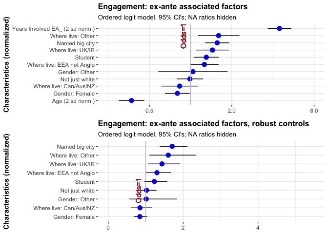
The results (for variables other than age and tenure are nearly identical, suggesting that these findings are not particularly sensitive to the functional form used to control for age and time in EA.*

* Recall: The USA is the base category for ‘where live,’ and ‘where live: other’ is outside Europe and Anglosphere, mainly Asia (top countries in this category: Israel, Singapore, China, Phillippines, Brazil, India, South Africa).

It is important to note that these are in multivariable models. Thus, while the odds-ratio shifter for ‘Where live: Other’ is among the most positive, this does not imply that the most-engaged EA’s are necessarily in these other countries.**

** This is probably not driven by our use of an ordered logit model; the linear model of the standardized 1-5 engagement measure finds a similar positive shift.

3.5.3.1 Selection and differential attrition: focus on recent recruits

We previously discussed how differential selection and attrition could drive the above models to suggest unwarranted predictions. We thus present a model isolating just those who say they became involved in 2019, 2018, or 2017. This includes most of ‘those with have been in EA less than the average duration.’ However it excludes those who joined in the survey year itself (2020), as those in their first year may be less able to gage their own engagment. We might suppose that the differential selection is less substantial over this shorter range of tenure. We might also imagine that patterns among ‘newer recruits’ are likely to be more reflective of future patterns. If so, the results below might be more predictive of engagement levels, and more useful for our ‘policy choices.’

newby_eas_20_s_imp <- eas_20_s_imp %>%
  filter(years_involved_d2sd < -0.001  & years_involved_d2sd > -0.5) %>%  #this captures people involved in 2018-2020
  mutate(year_involved = case_when( #recovering year_involved from trnasformed variable
    years_involved_d2sd < -.3  ~ "2019",
    years_involved_d2sd > -.3 & years_involved_d2sd < -.1  ~ "2018",
    years_involved_d2sd > -.1  ~ "2017"
        ),
    USA = where_live_cat=="USA"
  )


older_eas_20_s_imp <- eas_20_s_imp %>%
  filter(year_involved_groups  == "2014 or before" | year_involved_groups == "2015-16")  %>%  #this captures people involved in 2018-2020
  mutate(
    USA = where_live_cat=="USA"
  )

newby_ol_engage_imp <- newby_eas_20_s_imp %>%
    ol_mdl(c(key_predictors, "years_involved_d2sd"))

older_ol_engage_imp  <- older_eas_20_s_imp %>%
    ol_mdl(c(key_predictors, "years_involved_d2sd"))

newby_ol_engage_possible_endog <- newby_eas_20_s_imp %>%
    ol_mdl(c(key_predictors, "year_involved", possible_endog))

newby_ol_engage_possible_endog_USA <- newby_eas_20_s_imp %>%
    ol_mdl(c("age_approx_d2sd","gender_cat","student_cat", "race_cat","USA", "city_cat", "year_involved", possible_endog))

fh_imp_n <- newby_eas_20_s_imp %>% smn("first_hear")

newby_ol_engage_fh_imp <- newby_eas_20_s_imp %>%
    ol_mdl(c(key_predictors, "year_involved", fh_imp_n))

These models involve only 773 responses. As we are only considering three such tenure durations, we include a dummy for each ‘year first involved.’ Given the short tenure, we also do not anticipate that income or university rank could be particularly affected by EA engagement at this point; thus we focus on the larger set of features.

(
newby_ol_engage_possible_endog_tree <- newby_ol_engage_possible_endog %>%
        filter(!grepl("NA$",term)) %>%
 ggcoefstats(statistic=t,
              sort="ascending",
              stats.labels = "TRUE",
              title = "Engagement of those involved in 2017-19: associated factors ",
              subtitle = "Ordered logit, 95% CI's; 'Possibly endogenous features'; NA ratios hidden",
              vline=FALSE) +
  ggplot2::labs(
        x= NULL,
        y = "Characteristics (normalized)"
      ) +
      geom_vline(xintercept=1, colour="grey") +
    geom_text(aes(x=1, label="Odds=1", y=12), colour="brown", angle=90, vjust = -.9) +
      scale_x_continuous(limits=c(0, 4))
) %>%
  ggplotly

Making inferences from the above graph, we see greater self-reported engagement among:*

* As some of the confidence intervals for these odds ratios cross the threshold of unit (even) odds, these are not all statistically significant in a conventional sense. Nonetheless, one might reasonably update beliefs in this direction.

• Those located in a (named) big city
• UK and Ireland (and less so, the EEA)
• Non-‘western’ countries
• Those who attended high-ranked universities
• Students
• Younger people (the negative of “Age”)

(The above list is reported in approximate order of the magnitudes of these odds, also considering the tightness of the confidence bounds.)

We see less engagement for living in Canada, Australia, or New Zealand. (The base group, the USA is marginally less engaged; see other models).

Comparing a simpler model for those involved from 2017-2019 to a separate model for those involved in earlier years (both of these models use the linear time-in-EA control and the smaller, ex-ante set of variables):

(
newby_ol_engage_imp_tree <- newby_ol_engage_imp %>%
    filter(!grepl("NA$|Age|involve|Involved",term)) %>%
 ggcoefstats(statistic=t,
              sort="ascending",
              stats.labels = "TRUE",
              title = "Engagement of those involved in 2017-19: associated factors ",
              subtitle = "Ordered logit, 95% CI's; 'Ex-ante features'; NA ratios & age & tenure controls hidden",
              vline=FALSE) +
  ggplot2::labs(
        x= NULL,
        y = "Characteristics (normalized)"
      ) +
      geom_vline(xintercept=1, colour="grey") +
    geom_text(aes(x=1, label="Odds=1", y=5), colour="brown", angle=90, vjust = -.9) +
      scale_x_continuous(limits=c(0, 4.75))
) %>%
  ggplotly

(
older_ol_engage_imp_tree <- older_ol_engage_imp %>%
    filter(!grepl("NA$|Age|involve|Involved",term)) %>%
 ggcoefstats(statistic=t,
              sort="ascending",
              stats.labels = "TRUE",
              title = "Engagement of those involved before 2017...",
              vline=FALSE) +
  ggplot2::labs(
        x= NULL,
        y = "Characteristics (normalized)"
      ) +
      geom_vline(xintercept=1, colour="grey") +
    geom_text(aes(x=1, label="Odds=1", y=5), colour="brown", angle=90, vjust = -.9) +
      scale_x_continuous(limits=c(0, 4.75))
) %>%
  ggplotly()

(
  engage_newby_v_older <- ggarrange(newby_ol_engage_imp_tree, older_ol_engage_imp_tree,
                    ncol = 1, nrow = 2,
                    heights = c(1, 1),
                    align = "v",
                      common.legend = TRUE, legend = "bottom")
)

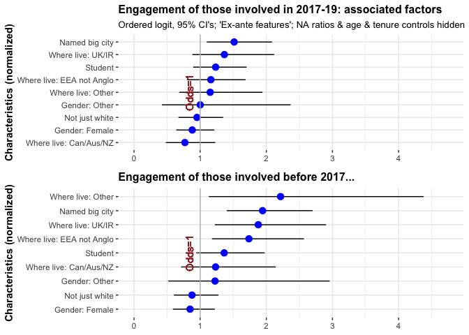
Although the confidence intervals are rather wide, especially for the longer tenure group, it looks fairly constant. The only major visual difference is that Can/Aus/NZ is ‘positive’ for those who joined in the earlier years (and persisted) and ‘negative’ for recent joiners. But again, this could be driven by differential selection.

Linear models (of levels and binary)

To consider the previous results’ sensitivity to functional form, we resent linear models considering:

1. self-reported engagement (engagement_num =1-5) as if it were a meaningful cardinal outcome, and also

2. the binary ‘highly engaged’ self-reported outcome of (‘4-5 engagement’ vs ‘1-3 engagement’)

#satis_ologit_t0 \<- eas_20 %\>% polr(m_f(sat_outcome, t0_satis_vars), data = ., Hess=TRUE) %\>%

#OK my 'coefficients as deviations' is not working. Back to the old crappy treatment coding with base groups as modal group in each case

#todo: get this to run with a *list* and with purrr, then easy switch to ologit

options(contrasts = rep("contr.treatment", 2))
#options(contrasts = rep ("contr.sum", 2))

lm_mdl <- function(df, rhs) {
  lm(
    m_f(num_out, {{rhs}}), data = df
    ) %>%
  lmtest::coeftest(vcov. = sandwich::vcovHC)
}

##Fix this -- its inheriting from outside the environment

lm_engage_naive <- eas_20_s_imp %>%
  lm_mdl(c(key_predictors))

  #lm(m_f(num_out, c("0", key_predictors)), data = .) %>%
  #lm(engagement_norm ~ 0 + gender_cat +  city_cat, data = .) %>%

lm_engage_noimp <- eas_20_s %>%
    lm_mdl(c(key_predictors, controls))

lm_engage_imp_big <- eas_20_s_imp %>%
  lm(m_f(num_out, c(big_demog,  controls)), data = .) %>%
  lmtest::coeftest(vcov = sandwich::vcovHC)

lm_engage_imp <- eas_20_s_imp %>%
    lm_mdl(c(key_predictors, controls))

lm_engage_possible_endog <- eas_20_s_imp %>%
    lm_mdl(c(key_predictors, controls, possible_endog))

fh_imp_n <- eas_20_s_imp %>% smn("first_hear")

lm_engage_fh_imp <- eas_20_s_imp %>%
    lm_mdl(c(key_predictors, controls, fh_imp_n))

key_pred_n_cat <- grep("first_hear_ea_lump|Intercept|NA|d2sd", names(coef(lm_engage_fh_imp)), value = TRUE, invert=TRUE)
na_pred <- grep("NA|Intercept", names(coef(lm_engage_fh_imp)), value = TRUE)
key_pred_n_ctn <- grep("d2sd", names(coef(lm_engage_fh_imp)), value = TRUE)
key_pred_n<- c(key_pred_n_ctn, key_pred_n_cat)


names(key_pred_n) <- gsub("d_live", "Live:", key_pred_n) %>%
  gsub("age_approx_d2sd", "Age (2sd norm)", .) %>%
  gsub("d2sd", " (norm)", .) %>%
  gsub("cat", "- ", .)  %>%
  #gsub("canzaus", "Aus///Can///NZ", .) %>%
  #gsub("d_", "", .) %>%
  gsub("_", " ", .)   %>%
  firstup(.)

fh_n <- grep("first_hear_ea_lump", names(coef(lm_engage_fh_imp)), value = TRUE)
names(fh_n) <- gsub("first_hear_ea_lump", "First-heard: ", fh_n)   %>%
    gsub("X80", "80", .)

huxreg_opts  <- function(df) {
 df %>%
    set_bold(1, everywhere)             %>%
    set_bottom_border(1, everywhere) %>%
    map_background_color(by_rows("grey87", "white"))  %>%
    set_caption_pos("bottom")
}

(
  lm_engage_tbl <- huxreg(
    "(0) Naive" = lm_engage_naive,
    "(1) Baseline " = lm_engage_imp, "(2) Baseline - no imputation" = lm_engage_noimp, "(3) Possibly endogenous" = lm_engage_possible_endog,  "(3) First-heard" = lm_engage_fh_imp,
      statistics = c("N. obs." = "nobs"),
    error_pos = "right",
    coefs = c(key_pred_n,  # note intercept was removed above
              "Income (norm)"= "income_d2sd",
              "Employed: Part-Time" = "d_pt_employment",
              "Not Employed" = "d_not_employed", "Retired" = "d_retired",
              fh_n)) %>%
        huxreg_opts %>%
    set_col_width(c(.5, rep(.2, times=length(.)-1)))
)

Table 3.2:

	(0) Naive		(1) Baseline		(2) Baseline - no imputation		(3) Possibly endogenous		(3) First-heard
Age (2sd norm)	-0.435 ***	(0.056)	-0.461 ***	(0.052)	-0.467 ***	(0.052)	-0.455 ***	(0.063)	-0.463 ***	(0.052)
Years involved (norm)			0.702 ***	(0.046)	0.703 ***	(0.047)	0.696 ***	(0.047)	0.696 ***	(0.049)
Gender - Female	-0.173 **	(0.055)	-0.100	(0.051)	-0.097	(0.052)	-0.103 *	(0.052)	-0.148 **	(0.052)
Gender - Other	0.095	(0.151)	0.020	(0.145)	0.024	(0.146)	0.006	(0.144)	-0.015	(0.144)
Student - Student	-0.052	(0.054)	0.130 *	(0.051)	0.117 *	(0.052)	0.141 *	(0.055)	0.108 *	(0.052)
Race - Not just white	-0.033	(0.058)	0.010	(0.055)	0.023	(0.056)	0.002	(0.056)	0.013	(0.056)
Where live - Can/Aus/NZ	-0.178 *	(0.084)	-0.097	(0.078)	-0.081	(0.079)	-0.108	(0.078)	-0.093	(0.079)
Where live - EEA not Anglo	0.052	(0.063)	0.103	(0.059)	0.108	(0.060)	0.103	(0.060)	0.079	(0.060)
Where live - Other	0.123	(0.091)	0.236 **	(0.086)	0.223 *	(0.090)	0.238 **	(0.086)	0.207 *	(0.087)
Where live - UK/IR	0.169 *	(0.072)	0.157 *	(0.067)	0.154 *	(0.067)	0.140 *	(0.069)	0.142 *	(0.069)
City - Named big city	0.295 ***	(0.052)	0.220 ***	(0.049)	0.227 ***	(0.050)	0.215 ***	(0.050)	0.207 ***	(0.049)
Income (norm)							-0.018	(0.070)
Employed: Part-Time							0.025	(0.101)
Not Employed							0.185	(0.108)
Retired							-0.003	(0.147)
First-heard: 80,000 Hours									-0.135	(0.077)
First-heard: Book, article, or blog post									0.042	(0.078)
First-heard: Educational course									0.246	(0.173)
First-heard: GiveWell									0.060	(0.153)
First-heard: Giving What We Can									-0.198	(0.178)
First-heard: LessWrong									-0.103	(0.085)
First-heard: Local or university EA group									0.077	(0.081)
First-heard: Personal contact									0.082	(0.068)
First-heard: Podcast									-0.069	(0.085)
First-heard: Slate Star Codex									-0.366 ***	(0.105)
First-heard: TED talk									0.092	(0.103)
N. obs.	1834		1834		1604		1834		1828
*** p < 0.001; ** p < 0.01; * p < 0.05.

(
  lm_engage_tbl_na <- huxreg(
    "(0) Naive" = lm_engage_naive,
    "(1) Baseline " = lm_engage_imp, "(2) Baseline - no imputation" = lm_engage_noimp, "(3) Possibly endogenous" = lm_engage_possible_endog,  "(3) First-heard" = lm_engage_fh_imp,
      statistics = c("N. obs." = "nobs"),
    error_pos = "right",
    coefs = c("(Intercept)", na_pred)) %>%
        huxreg_opts %>%
    set_col_width(c(.5, rep(.2, times=length(.)-1)))
)

Table 3.2:

	(0) Naive		(1) Baseline		(2) Baseline - no imputation		(3) Possibly endogenous		(3) First-heard
(Intercept)	0.002	(0.056)	-0.096	(0.053)	-0.097	(0.054)	-0.102	(0.056)	-0.044	(0.066)
gender_catNA	-0.153	(0.152)	-0.279 *	(0.142)	-0.248	(0.169)	-0.291 *	(0.142)	-0.263	(0.140)
student_catNA	-0.119	(0.193)	0.013	(0.173)	0.719	(0.525)	0.014	(0.175)	-0.018	(0.171)
race_catNA	-0.410 *	(0.195)	-0.285	(0.181)	-0.269	(0.252)	-0.276	(0.181)	-0.282	(0.180)
city_catNA	-0.048	(0.120)	-0.107	(0.114)	-0.189	(0.124)	-0.101	(0.115)	-0.080	(0.115)
N. obs.	1834		1834		1604		1834		1828
*** p < 0.001; ** p < 0.01; * p < 0.05.

Trying to automate the above

lm_mdl <- function(df, mod) {
  lm(
    m_f(num_out, {{rhs}}), data = df
    ) %>%
  coeftest(vcov = sandwich::vcovHC)
}


eng_models_list <- list(
    lm_engage_naive = 'm_f(num_out, c(key_predictors)',
    lm_engage_imp = 'm_f(num_out, c(big_demog,  "uni_higher_rank_d2sd", controls)'
  )

eng_model_frame <- tibble(model = eng_models_list) %>%
  mutate(model_name = names(model)) %>%
    mutate(model_name = names(model))

eng_model_frame <- eng_model_frame %>%
  mutate(fit = map(eng_model_frame,
                   ~lm(., data = eas_20_s_imp) %>%
                     coeftest(vcov = sandwich::vcovHC)
                     )
            )

Notes:

As in the Ordered Logit models, nonresponses for each response are included as separate categories. All “NA” coefficients are hidden. The outcome variable is standardized (de-meaned and divided by one SD).

Continuous variables (income, age, university rank) are de-meaned and divided by two standard-deviations. (This is for comparability to dummy-coded categorical variables, see Gelman [ref]) . Where these are missing they are coded as zero, the mean of the transformed variable (except in the “no imputation” column, where these are left out of the regression, leading to a smaller sample size.)

Base groups are set as the most numerous group in each category. All dummy coefficients represent adjustments from the ‘overall base group’: an individual who is Male, Works full-time, ‘Just White’ ethnicity, USA-based, not based in a (survey-named) big city, First heard of EA: ‘Other or don’t remember.’

3.6 Engagement: age, tenure, period and cohort effects

We examine the relationship between the year when people first got involved in EA (which tells us how long they’ve been in EA or their ‘tenure’), their current age and the age they were when they first got involved in EA.

See also “Tenure and ‘age first heard’ vs engagement” in demography chapter/post.

Aspirationally:

We would like to separate cohort, trend, and age effects here; we will have more possibility to do this if we combine data from earlier years.

“Engagement by years since joining, controlling for year and age”

“Engagement by year, controlling for years since joining and age”…

3.6.1 Engagement by tenure/age: ‘prediction for “outreach at what age?”’

A major concern might be: ‘What is the optimal age to reach out to EA’s?’

In a best-case we’d want to estimate the function (not ‘customer lifetime value’ but…) ‘effective lifetime value’ (\(ELV\)) as a function of ‘age first heard of EA’ (\(afh\)), and everything else (\(X\)): \[ELV = f(AFH, X)\]

and look for the values of AFH that maximizes this, perhaps averaging over the ‘everything else’ stuff.

Of course, we don’t know ELV, and it would take a great effort (as well as controversial assumptions) to construct this:

More simply, we could plot:

1. Engagement at age \(A\) as a function of age-first-heard (AFH):

This would combine both

• Tenure effects, as those who started younger have been in longer

  • and unfortunately, differentially attrited, adding a possible bias, and

• Receptiveness-at-age effects (e.g., earlier inculcation is stronger)

• Selection-at-age effects (e.g., those who we tend to recruit younger might be more engage-prone)

2. Engagement \(T\) years after first-heard as a function of AFH, combining

• Receptiveness-at-age effects (e.g., earlier inculcation is stronger)

• standard life-cycle age effects

• selection-at-age effects

3. Simple ‘engagement level by age’

• roughly capturing the life-cycle age effects
• but combining a variety of effects, including, e.g., ‘younger people might be more active,’ and ‘young people tend to have been in EA for less time’

3.6.2 Engagement by age and tenure

Below, we plot the ‘engagement level by age’ for the 2020 survey data…

#aet <- eas_20 %>% ungroup() %>%  dplyr::select(age_approx_ranges, engagement_num, tenure)

#p_load(scatterplot3d)

#scatterplot3d(eas_20$engagement, eas_20$age_approx, eas_20$tenure, highlight.3d=TRUE, col.axis="blue", col.grid="lightblue", main="scatterplot3d - 1", pch=20)
#ggExtra  to add densities

(
  engage_by_age <-  eas_20 %>%
  ggplot() +
  aes(x = age_approx, y = engagement_num) +
 geom_point(size = 0.30, colour = "#0c4c8a", position = position_jitter(seed = 42,  width = 0.1, height = 0.2)) +
 geom_smooth(span = 0.71) +
 scatter_theme +
 xlim(10L, 75L) +
    labs(y = get_label(eas_20$engagement_num),
         x = get_label(eas_20$age_approx))+
  labs(title = "Engagement (2020) by age")
) %>%
  ggplotly()

Looking at the average level of engagement of EAs of different ages, we observe a non-linear trend, with engagement flat or slightly increasing until the mid-to-late 20s and then declining. However, this should be expected to be strongly confounded with time-in-EA (or ‘tenure’), as EAs who have been in longer might be expected to be both older and more engaged than those who have joined EA more recently. (And age, being tied to year-first-involved, may also reflect differences in the cohorts introduced to EA).)

Noting this, we plot tenure against age below:

(
  tenure_by_age <-  eas_20 %>%
  ggplot() +
  aes(x = age_approx, y = tenure) +
 geom_point(size = 0.30, colour = "#0c4c8a", position = position_jitter(seed = 42,  width = 0.1, height = 0.2)) +
 geom_smooth(span = 0.71) +
scatter_theme +
xlim(10L, 75L) +
   labs(y = get_label(eas_20$tenure),
         x = get_label(eas_20$age_approx)) +
   labs(title = "Tenure by age (2020)")
) %>% ggplotly()

Indeed, tenure seems to increase steeply in age for ages below about 30. This could occur mechanically from an age-barrier to being introduced to EA; perhaps most people are not introduced to it until university.

Engagement by Age, ‘faceted’ by tenure (time in EA):

We also plot the relationship between age and average engagement for different groups of cohorts (0-1, 1-2, 2-3, 3-5 and 5-11 years in EA).

Here we still see a pattern of average engagement sharply increasing and then declining with increasing age. However, for each successively earlier set of cohorts (i.e. people who have been in EA longer), the peak age for engagement is commensurately older.

label_x <- function(p) {
  b <- ggplot_build(p)
  x <- b$plot$data[[b$plot$labels$x]]

  p + scale_x_continuous(
    attributes(x)$label,
    breaks = attributes(x)$labels,
    labels = names(attributes(x)$labels)
  )
}


(
engagement_by_age_facet_tenure <- eas_20 %>%
  ggplot() +
 aes(x = age_approx, y = engagement_num) +
 geom_point(size = 0.20, colour = "#0c4c8a", position = position_jitter(seed = 42,  width = 0.1, height = 0.2)) +
 geom_smooth(span = 0.71) +
scatter_theme +
 facet_grid(vars(), vars(tenure_ranges)) +
 xlim(10L, 75L) + ylim(0, 5.5) +
  labs(title = "Engagement by age",
    subtitle = "Faceted by time in EA") +
    labs(y = get_label(eas_20$engagement_num),
         x = get_label(eas_20$age_approx))
) %>%
  ggplotly()

Engagement appears to decrease in age for all tenure ranges. The peak of engagement is around 20-years-old.

However, this apparent ‘peak’ at age 20 may be illusory. Further data and modeling are needed (see note).

It might be that the age-20 thing is a ‘real peak’ (i.e., that people age 20 are more active than people age 18). But the CI’s are wide in the faceted data. To get a more precise estimate of ‘age 18’ vs ‘age 20’ (holding tenure constant) we need to look more carefully, within a model with, e.g., a linear tenure term Even within the tenure facets, there are variations in tenure, which may be driving the ‘bump at the beginning’ … those who are older still tend to have more tenure. (Also remember that this could be driven by a persistence/selection effect).

Engagement by tenure:

(
engagement_by_tenure_overall <-
  eas_20 %>%
  ggplot() +
  aes(x = tenure, y = engagement_num) +
 geom_point(size = 0.30, colour = "#0c4c8a", position = position_jitter(seed = 42,  width = 0.1, height = 0.2)) +
  geom_smooth(span = 0.75) +
  scatter_theme +
labs(title = "Engagement by time in EA") +
    labs(y = get_label(eas_20$tenure),
         x = get_label(eas_20$engagement_num))
) %>%
  ggplotly()

Engagement by tenure, ‘faceted’ by age groupings:

(
engagement_by_tenure_facet_age <-
  eas_20 %>%
  ggplot() +
  aes(x = tenure, y = engagement_num) +
 geom_point(size = 0.30, colour = "#0c4c8a", position = position_jitter(seed = 42,  width = 0.1, height = 0.2)) +
  geom_smooth(span = 0.75) +
  scatter_theme +
  facet_grid(vars(), vars(age_approx_ranges), scales = "free") +
labs(title = "Engagement by time in EA",
     subtitle = "Faceted by Age") +
    labs(y = get_label(eas_20$engagement_num),
         x = get_label(eas_20$tenure))

) %>%
  ggplotly

Engagement appears to increase in tenure for all age range (the ‘dip’ for the 26-29 age range has very wide confidence intervals and appears driven by a few observations). The slope appears particular positive in the first few years. However, given that this is recall data (2020 retrospective only), we cannot rule out that this is driven by a selectivity effect (only those who are engaged choose to persist).

We plot this again on a single graph:

(engage_age_group_tenure <-
eas_20 %>%
  ggplot() +
  aes(x = age_approx, y = engagement_num, colour = tenure_ranges, group = tenure_ranges) +
  geom_point(size = 0.20, colour = "#0c4c8a",
            position = position_jitter(seed = 42,  width = 0.1, height = 0.2)) +
    geom_smooth(span = 0.71, se=F) +
  scatter_theme +
  xlim(15L, 75L) +
  ylim(0, 5.5) +
  labs(title = "Engagement by age, grouped by tenure:")
)  %>%
  ggplotly

3.6.3 Engagement by ‘Age-first-involved’ and tenure

Below, we also depict each of the above graphs in terms of ‘age-first-involved’ (AFI) and tenure. Note again that, as we are only using 2020 recall data here, \(tenure = 2020 - year\_first\_involved\). Thus, this simply implies a re-labeling and a shifting, as seen below.

(
  engage_by_age_first_involved <-  eas_20 %>%
  ggplot() +
  aes(x = age_first_inv, y = engagement_num) +
 geom_point(size = 0.20, colour = "#0c4c8a", position = position_jitter(seed = 42,  width = 0.1, height = 0.2)) +
 geom_smooth(span = 0.71) +
 theme_minimal() +
 xlim(10L, 75L) +
  labs(title = "Engagement by age first involved")
)  %>%
  ggplotly

require("ggpubr")
(
  figure <- ggarrange(engage_by_age_first_involved, engage_by_age,
                    ncol = 2, nrow = 1,
                    heights = c(1, 1),
                    align = "v",
                      common.legend = TRUE, legend = "bottom")
)

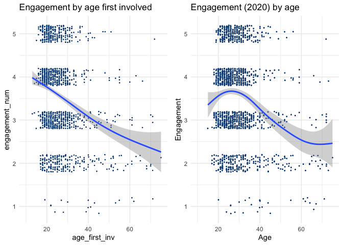
Engagement by age first involved, faceted by tenure:

(
engagement_by_afi_facet_tenure <- eas_20 %>%
  ggplot() +
 aes(x = age_first_inv, y = engagement_num) +
 geom_point(size = 0.20, colour = "#0c4c8a", position = position_jitter(seed = 42,  width = 0.1, height = 0.2)) +
 geom_smooth(span = 0.71) +
scatter_theme +
  facet_grid(vars(), vars(tenure_ranges)) +
 xlim(10L, 75L) +
 ylim(0, 5.5) +
labs(title = "Engagement by age first involved, faceted by tenure",
     subtitle = "Faceted by time in EA") +
    labs(y = get_label(eas_20$engagement_num),
         x = get_label(eas_20$age_first_inv))
)

(
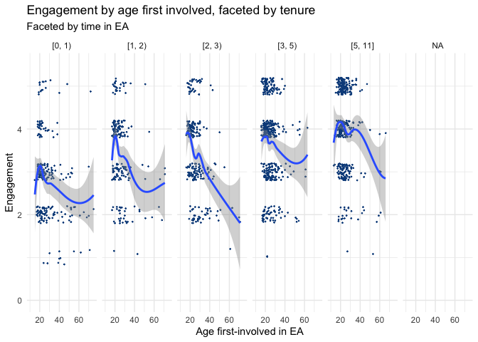
  engage_afi_vs_age_facet_tenure <- ggarrange(engagement_by_afi_facet_tenure, engagement_by_age_facet_tenure,
                    ncol = 1, nrow = 2,
                    heights = c(1, 1),
                    align = "v",
                      common.legend = TRUE, legend = "bottom")
)

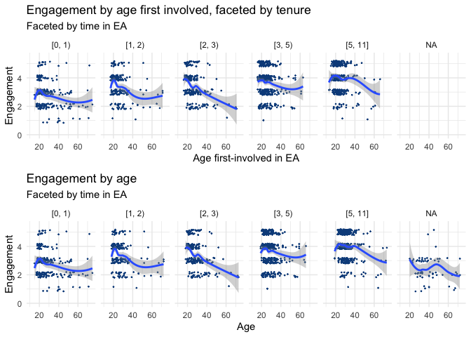
Note that above, these are simply shifted versions of the same graphs.*

* I prefer the bottom graph, as I suspect that that ‘age’ is the more important thing to emphasise.

I suspect that, holding tenure constant… … life-cycle-age: “I’m now 20, so I can be active vs. I’m 35 and I have a mortgage and 4 kids” plays a greater effect than

• “receptivity at the age when I joined EA” (‘I got involved at 20 when I was impressionable’)

Next, the ‘effect’ of tenure, faceted by age first involved (vs. age)

engagement_by_tenure_facet_afi <-
  eas_20 %>%
  ggplot() +
  aes(x = tenure, y = engagement_num) +
 geom_point(size = 0.30, colour = "#0c4c8a", position = position_jitter(seed = 42,  width = 0.1, height = 0.2)) +
  geom_smooth(span = 0.75) +
  ggthemes::theme_solarized_2() +
 facet_grid(vars(), vars(age_first_inv_ranges), scales = "free") +
  labs(title = "Engagement by tenure, faceted by age-first-involved")


(
  engagement_by_tenure_facet_afi_vs_age <- ggarrange(engagement_by_tenure_facet_afi, engagement_by_tenure_facet_age,
                    ncol = 1, nrow = 2,
                    heights = c(1, 1),
                    align = "v",
                      common.legend = TRUE, legend = "bottom")
)

The above graphs differ only slightly, as the definition of the quantiles used for faceting are slightly different.

Finally, the analogue to the grouped (single-graph) plots:

engage_afi_group_tenure <-
eas_20 %>%
  ggplot() +
  aes(x = age_first_inv, y = engagement_num, colour = tenure_ranges, group = tenure_ranges) +
  geom_point(size = 0.20, colour = "#0c4c8a",
            position = position_jitter(seed = 42,  width = 0.1, height = 0.2)) +
    geom_smooth(span = 0.71, se=F) +
  theme_minimal() +
  xlim(15L, 75L) +
  ylim(0, 5.5) +
  labs(title = "Engagement by age-first-involved, grouped by tenure:")



(
  engage_afi_vs_age_group_tenure <- ggarrange(engage_afi_group_tenure, engage_age_group_tenure,
                    ncol = 2, nrow = 1,
                    heights = c(1, 1),
                    align = "h", legend = "bottom")
)

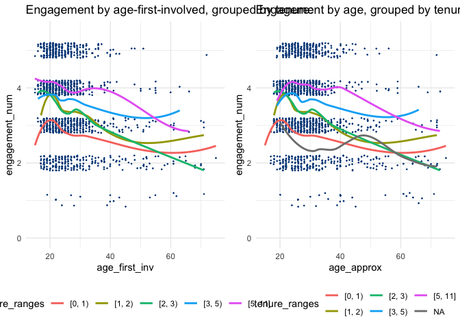
The above graphs are nearly identical but for the slight shift in the x-axis, and the inclusion of the NA tenure-range category (we cannot infer age-first-involved where individual’s did not answer this question).*

* There also seem to be some very small differences in the shape of the smoothed plots; this might result from a quirk in the smoothing algorithm, or some rounding issue, I am not sure.

3.6.4 See also: Attrition from EA/EA survey by introducer

3.7 Additional – CEA request: cities/areas by group engagement and retention, adapted:

(
retain_engage_by_area <- eas_20 %>%
  mutate(
    city = as.character(city),
    country = as.character(country),
    cea_region_selection = case_when(
      str_detect(city, "London|New York|SF Bay|DC") ~ city,
      str_detect(country, "Netherlands|Germany") ~ country,
    TRUE ~ "Other",
      ),
    group_made_more_engaged = as.numeric(engaged_local_groups=="Made me a lot more likely to stay engaged"|engaged_local_groups=="Made me more likely to stay engaged")
    )  %>%
  filter(!is.na(engaged_local_groups)) %>%
 ggplot() +
 aes(x = reorder(cea_region_selection, group_made_more_engaged) ) +
  geom_bar(aes(fill=engaged_local_groups), position="fill")  +
  stat_summary(aes(y = group_made_more_engaged),
           fun.data = mean_cl_normal,  na.rm = TRUE,
           geom = "errorbar", colour = "white", width = 0.35) +
stat_summary(aes(y = group_made_more_engaged),
           fun.data = mean_cl_normal,  na.rm = TRUE,
           geom = "errorbar",  colour = "brown", width = 0.35,
           fun.args = list(mult = 1)) +
  theme(axis.text.x = element_text(angle = 90, vjust = 0.5, hjust=1)) +
    labs(title = "'Impact of groups on engagement' by select areas", x="City/country", y="share", caption = "95% CI bars for 'Made more/ a lot more likely' in white, 1 SE in brown") +
     coord_flip(ylim = c(0, 1))
)

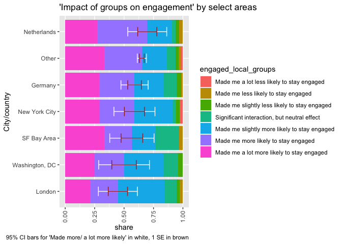
Above, for a select list requested by CEA. Note that this excludes some larger cities and countries.

The above should be treated cautiously. There are several other things wrong with the inferences one might draw from this analysis.

• Differential selection (e.g., one city’s EA group is very insular and exclusive, so only those who are really in the clique join it and report high levels)

• Differential baseline characteristics of EA’s in different cities

3.8 Conclusions and Future work

This post has presented a descriptive picture of the ways EAs engage, how they rate their own engagement, and how these relate to other attitudes and observable characteristics. This broadly aids our understanding of “what engagement in the EA movement looks like” and “who/what/where” EA’s engage.

Summarizing some of our findings (unfold)

• Self-reported engagement is strongly associated with membership in EA groups and with taking more EA-relevant actions, arguing for the validity of this measure
• ‘Engagement tends to decrease in age after age-20 but increase with time-in-EA’
• People reporting that they ‘first heard of EA’ from certain sources (such as “Educational Courses, and Personal Contact” tend to have higher engagement than average, even after controlling for factors like age and time-in-EA
• Those living in the (named) big cities, as well as certain geographic regions tend to have higher engagement than average, even after controlling for other factors

However, given our retrospective data, many of these differences could reflect differential attrition processes between groups, as discussed above.

In addition to description, we are also interested in more ambitious predictive and even causal modeling of engagement for several reasons. As discussed in the supplement [LINK], we may care about (i) Outreach, (ii) Planning, and (iii) Policy. Key questions include

1. Which types of people are more or less likely to become engaged in EA, and how does this inform EA organizations’ optimal outreach strategies, if at all?

2. What approaches lead people to become more involved in EA?

3. How large is the EA movement likely to grow over time, and what levels (and types) of engagement  can predict this? This could inform our plans for building infrastructure, as well as our impact strategies and approaches. 

We suspect that more in-depth analysis of these issues is warranted, and we hope to pursue this going forward. For example:, 

• We are working to bring together the EA survey data across years, allowing us to separate “time in EA” from “year joined EA,” and perform “Age-Period-Cohort” analysis.

  • Considering “movement growth”: We hope to combine this with medium-term prediction models explicitly quantifying our uncertainty into probabilistic forecasts of key outcomes.

• We aim to build (ML) models to predict engagement outcomes from initially-observable characteristics. 

  • In particular, we could initial characteristics/responses from earlier EAS data to predict presence in later surveys, as one measure of engagement. (We can connect some participants across surveys through anonymized emails.)

We expect causal inference, learning what approaches would “make people become more involved,” will  be more difficult. Key explanatory variables are entangled, and were not ‘experimentally assigned’: the ways that people are introduced to EA, the groups they are associated with, their experiences, and the ways that EA groups and organizations interact with members, etc. Nonetheless, further analysis, using techniques from the fields of causal inference, statistics, and econometrics, may allow us to make some reasonable causal inferences

3.8.1 Future engagement and retention modeling (after forum-post additions)

• see Ben West post

• CEA published a new analysis of retention based on their own data https://forum.effectivealtruism.org/posts/TeCsTp7pZPFQtJhme/estimates-of-highly-engaged-ea-retention

3.9 After-post followups/further work

3.9.1 Does engagement in EA make people more long-termist?

From post:

As we can see, average support for Near-termist causes declines with increases in engagement, while support for Longtermist and Meta causes increases.

Question from Arepo

I would love to see research into the direction of causality here. I think it’s very easy to assume engagement drives the realisation of belief in longtermism, and much EA messaging supports this - eg Will’s(?) statement that longtermism might be the biggest breakthrough of the EA movement. But I know many people for whom it seemed to run the other way - they lost interest over time in part because of the movement’s obsession with replacing concrete short term value with (as they see it) motivated speculation.

We can separate at possible mechanisms that might be driving the above observation; we may seek to measure to what extent:

1. Engagement \(\rightarrow\) Lt-ism: Time spent in EA and/or engagement in EA leads people to become more long-termist?

2. LT-ism \(\rightarrow\) engagement: People who are less long-termist become less engaged and/or drop out?

In measuring this, we need to consider underlying year-on-year trends that may complicate estimation:

3. Trends to Lt-ism in the underlying population: Considering any fixed group of potential recruits (e.g., those people that would have joined EA in 2015). This group may themselves be becoming more (or less) LT-ist over the years, even before exposure to EA.

4. Differential (self) selection of recruits over time: As the EA movement trends to LT-ism, people who are less long-termist are less likely to join.

Approaches to answering this

For 2.  LT-ism –> Engagement: (?) 

A. With ‘connected data’ we could measure whether those in the earlier years’ data who express LT-ist attitudes are more likely to appear in later years’ data, and to be more engaged

(this relates to a ‘next project’ we are discussing and working on)

B. Even with unconnected multi-year data we can consider people coming from groups that… presumably are likely to be more LT-ist (‘first-heard = LessWrong’ etc.)
…coming from the same cohorts (e.g., joined EA in 2015) … get bigger or smaller across EA surveys, relative to less-LT-ist-seeming groups (And we could do the same for ‘number of 4+ engaged’ in each group) … E.g., suppose the cohort “joined in 2015, heard of EA from GWWC” shrinks from 2017-2020, while the cohort “joined in 2015, heard of EA from LW” increases … this may suggest less-LT-ist people are dropping out more.

(But all of this assumes that dropout from the survey is proportional to dropout from the movement)

#From https://stackoverflow.com/questions/62028925/how-do-i-catch-errors-in-inline-code-chunk-in-r-markdown

knitr::knit_hooks$set(
  evaluate.inline = function (code, envir = knit_global()) {
    v = try(eval(xfun::parse_only(code), envir = envir))
    knitr::knit_print(v, inline = TRUE, options = knitr::opts_chunk$get())
  },
  inline = function(x) {
  if (any(class(x) == "try-error")) {
    as.vector(x)
  } else x
})

# knitr::knit_hooks$set(inline = function(x) {
#   if(is.double(x))
#   x <- sprintf("%1.1f", x)
# })